Linear Regression and Optimisation
When I first learnt linear regression six years ago, I was surprised by its power. I could know the effect of one phenomenon on another and the extent of the relationship. As years passed by, I revisited its different parts in pieces. Stability. Consistency. Precision. R Squared. The list goes on.
Sometime in the past, I decided to compile all I had learnt about linear regression. However, such massive projects never see fruition. In my MBA, Prof Amlesh Sharma from Texas A&M taught this in his Advanced Marketing Analytics class; I didn’t find this technique elsewhere. Using this simple trick, you can decide the optimal value for input to produce the maximum output.
Formulation
At its heart, linear regression is fitting a straight line in the existing data so that the line is closest to the points. We solve the optimisation problem to minimise the distance between the regression line and the actual observation. This approach is called “loss minimisation”. Another popular method is to “maximise likelihood”. Explanation of these methods is beyond the scope of this article.
Variables
Independent variables (X): Independent variables are assumed to be independent of each other and the cause of an effect.
Dependent variable (Y): Dependent variable is the final effect we try to estimate or predict.
Case Study: Number of Golf Courses
There is a strong theoretical reason to believe that the number of golf courses in a state would depend on climate, population, per capita income and popularity. Consider a simple case where you know only the people of the state and the number of golf courses in that state.
The linear model to find the number of gold courses can be written as the following.
\[ Y = \beta_0 + \beta_1X \varepsilon \]
\(Y\) is the number of golf courses in the state and \(X\) is population.
Is the relationship linear?
Let’s check it.
Data
Data on golf courses by US state is available at this website. I scrapped it into a .CSV file available here.
library(tidyverse)## ── Attaching core tidyverse packages ──────────────────────── tidyverse 2.0.0 ──
## ✔ dplyr 1.1.2 ✔ readr 2.1.4
## ✔ forcats 1.0.0 ✔ stringr 1.5.0
## ✔ ggplot2 3.4.3 ✔ tibble 3.2.1
## ✔ lubridate 1.9.2 ✔ tidyr 1.3.0
## ✔ purrr 1.0.2
## ── Conflicts ────────────────────────────────────────── tidyverse_conflicts() ──
## ✖ dplyr::filter() masks stats::filter()
## ✖ dplyr::lag() masks stats::lag()
## ℹ Use the conflicted package (<http://conflicted.r-lib.org/>) to force all conflicts to become errorstheme_set(theme_h())
golf = read.csv("https://www.harsh17.in/using-linear-regression-to-find-optimal-value/data/golf.csv") %>% as_tibble()
golf## # A tibble: 52 × 4
## State Location.quotient Establishments Employment
## <chr> <dbl> <chr> <chr>
## 1 U.S. Total 1 11,088 306,782
## 2 Florida 2.66 884 48,670
## 3 Hawaii 2.5 57 3,491
## 4 South Carolina 2.1 256 9,094
## 5 Arizona 1.58 168 9,417
## 6 Nevada 1.39 83 3,959
## 7 North Carolina 1.35 402 12,496
## 8 Alabama 1.14 150 4,670
## 9 Pennsylvania 1.13 551 13,975
## 10 Georgia 1.1 279 10,279
## # ℹ 42 more rowsPopulation of each US state is available on this website. I downloaded the .CSV file available from there (click here to download).
population = read.csv("https://www.harsh17.in/using-linear-regression-to-find-optimal-value/data/state_population.csv") %>% as_tibble()
population
## # A tibble: 52 × 9
## rank State Pop Growth Pop2021 Pop2010 growthSince2010 Percent density
## <int> <chr> <int> <dbl> <int> <int> <dbl> <dbl> <dbl>
## 1 1 Califor… 3.97e7 0.0013 3.96e7 3.73e7 0.0628 0.118 255.
## 2 2 Texas 3.01e7 0.0124 2.97e7 2.52e7 0.192 0.0896 115.
## 3 3 Florida 2.22e7 0.0106 2.19e7 1.88e7 0.177 0.066 414.
## 4 4 New York 1.92e7 -0.004 1.93e7 1.94e7 -0.0091 0.0572 408.
## 5 5 Pennsyl… 1.28e7 0.0001 1.28e7 1.27e7 0.0074 0.0381 286.
## 6 6 Illinois 1.25e7 -0.0041 1.26e7 1.28e7 -0.0251 0.0372 225.
## 7 7 Ohio 1.17e7 0.0011 1.17e7 1.15e7 0.0163 0.0349 287.
## 8 8 Georgia 1.09e7 0.0098 1.08e7 9.71e6 0.126 0.0325 190.
## 9 9 North C… 1.08e7 0.0099 1.07e7 9.57e6 0.129 0.0322 222.
## 10 10 Michigan 1.00e7 0.0003 9.99e6 9.88e6 0.0119 0.0297 177.
## # ℹ 42 more rowsNote that there is a timeline mismatch. Golf course data is from 2017, and population data is from 2021. However, since the purpose of this article is to show linear regression-based optimisation and not an actual world application — it’s acceptable.
Wrangling Data
Let’s merge the two datasets and retain only the columns that we need.
# inner join
df = inner_join(golf, population)
## Joining with `by = join_by(State)`# retain only number of golf courses and population in 2021
df = df %>%
select(State, Establishments, Pop2021)
# Establishments is in characters, so convert it to numeric
df$Establishments = as.numeric(df$Establishments)Visualisation
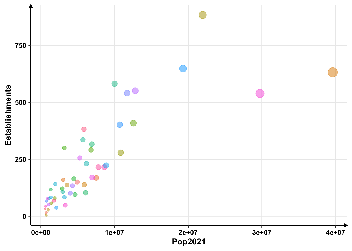
Just out of curiosity, let’s see how number of golf courses are with respect to state population.
df %>%
  ggplot(aes(x = Pop2021, y = Establishments, colour = State, size = Pop2021)) +
  geom_point(alpha = 0.5, show.legend = FALSE)
So there is a straightforward pattern that as the population increases, the number of golf courses increases. However, the variance also increases with population. When the population is around 20 million, golf courses can be about 600 or 800. There will likely be heteroskedasticity problems because of dependent variance if we directly apply a linear model.
Optimisation
Imagine if I rewrite the linear model differently.
\[ Y = a + bX + cX^2 \]
\(Y\) is the number of golf courses and \(X\) is the population.
Then, I can calculate \(\frac{dY}{dX}\) as the following.
\[ \frac{dY}{dX} = b + 2cX \]
For the optimal value — minimum or maximum — we will set the first order condition to zero. Thus,
\[ X = \frac{-b}{2c}. \]
Whether it will give us minima or maxima will depend on sign of \(\frac{d^2Y}{dX^2} = 2c\), i.e. sign of \(c\). So, let’s first estimate the model and see what we get.
fit = lm(Establishments ~ Pop2021 + I(Pop2021^2), data = df)
summary(fit)
##
## Call:
## lm(formula = Establishments ~ Pop2021 + I(Pop2021^2), data = df)
##
## Residuals:
## Min 1Q Median 3Q Max
## -154.203 -48.364 2.627 41.706 244.067
##
## Coefficients:
## Estimate Std. Error t value Pr(>|t|)
## (Intercept) -1.070e+01 2.219e+01 -0.482 0.632
## Pop2021 4.648e-05 4.580e-06 10.149 1.55e-13 ***
## I(Pop2021^2) -7.671e-13 1.328e-13 -5.778 5.46e-07 ***
## ---
## Signif. codes: 0 '***' 0.001 '**' 0.01 '*' 0.05 '.' 0.1 ' ' 1
##
## Residual standard error: 87.98 on 48 degrees of freedom
## Multiple R-squared: 0.8092, Adjusted R-squared: 0.8013
## F-statistic: 101.8 on 2 and 48 DF, p-value: < 2.2e-16We see that \(c = -7.6 \times 10^{-13}\), which is negative. Thus, the value we get from \(X = \frac{-b}{2c}\) will be maximiser. At that population, we would have the maximum number of golf courses.
Let’s calculate that critical value.
cc = coef(fit)
print(unname(-cc[2]/(2*cc[3])))
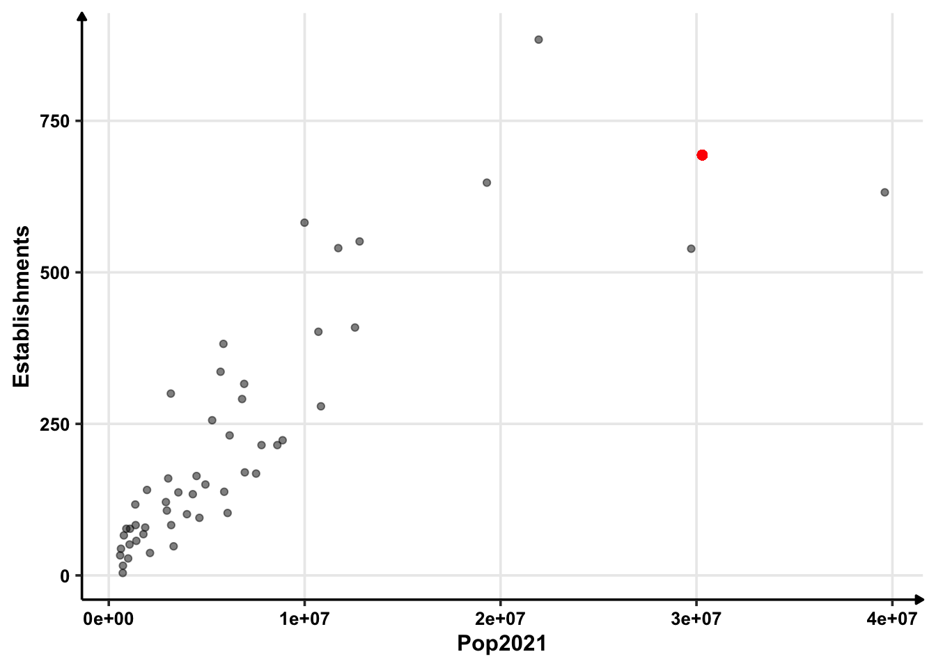
## [1] 30296969X = -cc[2]/(2*cc[3])Thus, the population that maximises the number of golf courses is 30,296,969 — around thirty million.
How many golf courses we will have in that case?
(Y = cc %*% c(1, X, X^2))## [,1]
## [1,] 693.4493It will have around 694 golf courses. This looks like a correct answer from the plot as well.
df %>%
  ggplot(aes(x = Pop2021, y = Establishments)) +
  geom_point(alpha = 0.5) +
  geom_point(aes(X, Y), colour = "red", size = 2)