Titanic: Who Survived The Tragedy?

Titanic was a major tragedy. In this course project for BZAN 645: Machine Learning at University of Tennessee, I tried to predict if a particular individual would survive the tragedy. Why Titanic Dataset? Because it was course requirement. No offence to hundreds of soul that died, but the dataset is easy to get started with. Every course instructor loves it.
I used Tidymodels to use xgboost and logistic regression with bootstrapped samples to predict the outcome.
Loading Libraries and Dataset
# Setting Parallel Processing to use six out of eight cores
# Unix and macOS only
library(doMC)
## Loading required package: foreach

## Loading required package: iterators

## Loading required package: parallel
registerDoMC(cores = 6)

# To reset, use
# registerDoSEQ()
library(tidyverse)
## ── Attaching packages ─────────────────────────────────────── tidyverse 1.3.1 ──

## ✓ ggplot2 3.3.5          ✓ purrr   0.3.4
## ✓ tibble  3.1.6          ✓ dplyr   1.0.8.9000
## ✓ tidyr   1.2.0          ✓ stringr 1.4.0
## ✓ readr   2.1.2          ✓ forcats 0.5.1

## ── Conflicts ────────────────────────────────────────── tidyverse_conflicts() ──
## x purrr::accumulate() masks foreach::accumulate()
## x dplyr::filter()     masks stats::filter()
## x dplyr::lag()        masks stats::lag()
## x purrr::when()       masks foreach::when()
library(tidymodels)
## Registered S3 method overwritten by 'tune':
##   method                   from
##   required_pkgs.model_spec parsnip

## ── Attaching packages ────────────────────────────────────── tidymodels 0.1.4 ──

## ✓ broom        0.7.10     ✓ rsample      0.1.1
## ✓ dials        0.0.10     ✓ tune         0.1.6
## ✓ infer        1.0.0      ✓ workflows    0.2.4
## ✓ modeldata    0.1.1      ✓ workflowsets 0.1.0
## ✓ parsnip      0.1.7      ✓ yardstick    0.0.9
## ✓ recipes      0.1.17

## ── Conflicts ───────────────────────────────────────── tidymodels_conflicts() ──
## x purrr::accumulate() masks foreach::accumulate()
## x scales::discard()   masks purrr::discard()
## x dplyr::filter()     masks stats::filter()
## x recipes::fixed()    masks stringr::fixed()
## x dplyr::lag()        masks stats::lag()
## x yardstick::spec()   masks readr::spec()
## x recipes::step()     masks stats::step()
## x purrr::when()       masks foreach::when()
## • Search for functions across packages at https://www.tidymodels.org/find/
library(plotly)
##
## Attaching package: 'plotly'

## The following object is masked from 'package:ggplot2':
##
##     last_plot

## The following object is masked from 'package:stats':
##
##     filter

## The following object is masked from 'package:graphics':
##
##     layout
# Setting custom theme
theme_h = function(base_size = 14) {
  theme_bw(base_size = base_size) %+replace%
    theme(
      # Specify plot title
      plot.title = element_text(size = rel(1), face = "bold", family="serif", margin = margin(0,0,5,0), hjust = 0),
      # Specifying grid and border
      panel.grid.minor = element_blank(),
      panel.border = element_blank(),
      # Specidy axis details
      axis.title = element_text(size = rel(0.85), face = "bold", family="serif"),
      axis.text = element_text(size = rel(0.70), family="serif"),
      axis.line = element_line(color = "black", arrow = arrow(length = unit(0.3, "lines"), type = "closed")),
      # Specify legend details
      legend.title = element_text(size = rel(0.85), face = "bold", family="serif"),
      legend.text = element_text(size = rel(0.70), face = "bold", family="serif"),
      legend.key = element_rect(fill = "transparent", colour = NA),
      legend.key.size = unit(1.5, "lines"),
      legend.background = element_rect(fill = "transparent", colour = NA),
      # Remove default background
      strip.background = element_rect(fill = "#17252D", color = "#17252D"),
      strip.text = element_text(size = rel(0.85), face = "bold", color = "white", margin = margin(5,0,5,0), family="serif")
    )
}

theme_set(theme_h())
You can download the datasets here.
xfun::embed_file(path = "/Users/harshvardhan/Documents/UTK/Classes/Spring 2022/BZAN 645 Machine Learning/Homeworks/HW03/titanic-tidymodels/train.csv")
xfun::embed_file(path = "/Users/harshvardhan/Documents/UTK/Classes/Spring 2022/BZAN 645 Machine Learning/Homeworks/HW03/titanic-tidymodels/test.csv")
training = read_csv("/Users/harshvardhan/Documents/UTK/Classes/Spring 2022/BZAN 645 Machine Learning/Homeworks/HW03/titanic-tidymodels/train.csv")
## Rows: 891 Columns: 12
## ── Column specification ────────────────────────────────────────────────────────
## Delimiter: ","
## chr (5): Name, Sex, Ticket, Cabin, Embarked
## dbl (7): PassengerId, Survived, Pclass, Age, SibSp, Parch, Fare
##
## ℹ Use `spec()` to retrieve the full column specification for this data.
## ℹ Specify the column types or set `show_col_types = FALSE` to quiet this message.
testing = read_csv("/Users/harshvardhan/Documents/UTK/Classes/Spring 2022/BZAN 645 Machine Learning/Homeworks/HW03/titanic-tidymodels/test.csv")
## Rows: 418 Columns: 11
## ── Column specification ────────────────────────────────────────────────────────
## Delimiter: ","
## chr (5): Name, Sex, Ticket, Cabin, Embarked
## dbl (6): PassengerId, Pclass, Age, SibSp, Parch, Fare
##
## ℹ Use `spec()` to retrieve the full column specification for this data.
## ℹ Specify the column types or set `show_col_types = FALSE` to quiet this message.
training
## # A tibble: 891 × 12
##    PassengerId Survived Pclass Name   Sex     Age SibSp Parch Ticket  Fare Cabin
##          <dbl>    <dbl>  <dbl> <chr>  <chr> <dbl> <dbl> <dbl> <chr>  <dbl> <chr>
##  1           1        0      3 Braun… male     22     1     0 A/5 2…  7.25 <NA>
##  2           2        1      1 Cumin… fema…    38     1     0 PC 17… 71.3  C85
##  3           3        1      3 Heikk… fema…    26     0     0 STON/…  7.92 <NA>
##  4           4        1      1 Futre… fema…    35     1     0 113803 53.1  C123
##  5           5        0      3 Allen… male     35     0     0 373450  8.05 <NA>
##  6           6        0      3 Moran… male     NA     0     0 330877  8.46 <NA>
##  7           7        0      1 McCar… male     54     0     0 17463  51.9  E46
##  8           8        0      3 Palss… male      2     3     1 349909 21.1  <NA>
##  9           9        1      3 Johns… fema…    27     0     2 347742 11.1  <NA>
## 10          10        1      2 Nasse… fema…    14     1     0 237736 30.1  <NA>
## # … with 881 more rows, and 1 more variable: Embarked <chr>
testing
## # A tibble: 418 × 11
##    PassengerId Pclass Name   Sex     Age SibSp Parch Ticket  Fare Cabin Embarked
##          <dbl>  <dbl> <chr>  <chr> <dbl> <dbl> <dbl> <chr>  <dbl> <chr> <chr>
##  1         892      3 Kelly… male   34.5     0     0 330911  7.83 <NA>  Q
##  2         893      3 Wilke… fema…  47       1     0 363272  7    <NA>  S
##  3         894      2 Myles… male   62       0     0 240276  9.69 <NA>  Q
##  4         895      3 Wirz,… male   27       0     0 315154  8.66 <NA>  S
##  5         896      3 Hirvo… fema…  22       1     1 31012… 12.3  <NA>  S
##  6         897      3 Svens… male   14       0     0 7538    9.22 <NA>  S
##  7         898      3 Conno… fema…  30       0     0 330972  7.63 <NA>  Q
##  8         899      2 Caldw… male   26       1     1 248738 29    <NA>  S
##  9         900      3 Abrah… fema…  18       0     0 2657    7.23 <NA>  C
## 10         901      3 Davie… male   21       2     0 A/4 4… 24.2  <NA>  S
## # … with 408 more rows
Here’s a brief overview of the variables:
PassengerIdidentifies the variable. This is not useful for our model.Survivedis a binary variable indicating if the passenger survived.Pclasstell us the class of passenger. We will have to perform one hot encoding for this variable.Nameis the name of the passenger. This is not useful for our model.Sexis the sex of passenger. This will also need to be one-hot-encoded.Ageis the age of passenger. Those in decimals are estimated ages. In our model, we will treat it like a continuous variable.SibSpis the number of siblings or spouses on the ship. (I wonder if Jack counted as Rose’s spouse but probably not as their relationship only began on the ship.)Parchis the number of parents or children abroad the ship.Ticketis a character variable with the ticket’s serial number.Fareis the amount paid for fare.Cabinnumbers are largely missing.Embarkedis the location the passengers boarded the ship. This will also need to be one-hot-encoded.
Exploring Dataset
Missing Values
missing_df = function(df)
{
   nf = ncol(df)
   miss_rate = numeric(nf)
   for (i in 1:nf)
   {
      miss_rate[i] = sum(is.na(df[,i]))/nrow(df)
   }
   ll = tibble("names" = names(df), "miss_rate" = miss_rate)
   return(ll)
}
missing_df(training)
## # A tibble: 12 × 2
##    names       miss_rate
##    <chr>           <dbl>
##  1 PassengerId   0
##  2 Survived      0
##  3 Pclass        0
##  4 Name          0
##  5 Sex           0
##  6 Age           0.199
##  7 SibSp         0
##  8 Parch         0
##  9 Ticket        0
## 10 Fare          0
## 11 Cabin         0.771
## 12 Embarked      0.00224
Age has lots of missing variables and Cabin has many missing values. Embarked has a few missing values. I should probably drop Cabin from analysis, and impute values for the other two.
So, three alternatives:
- Delete the observations with missing values,
- Impute missing values with mean (for numeric) and mode (for categorical),
- Remove variables Age, Cabin and Embarked altogether.
Number of Survivors
First, we will test for class imbalance. Did more people survive than die, or vice versa?
training %>%
   count(Survived)
## # A tibble: 2 × 2
##   Survived     n
##      <dbl> <int>
## 1        0   549
## 2        1   342
The classes are almost balanced. 342 people survived; 549 didn’t.
Class of Passengers (and Survivors)
training %>%
   count(Pclass)
## # A tibble: 3 × 2
##   Pclass     n
##    <dbl> <int>
## 1      1   216
## 2      2   184
## 3      3   491
Most passengers were travelling in the third class.
training %>%
   count(Pclass, Survived) %>%
   ggplot(aes(x = Pclass, y = n, fill = factor(Survived))) +
   geom_bar(position = "stack", stat="identity") +
   labs(x = "Class of Passenger", y = "Number of Passengers",
        fill = "Survived?")
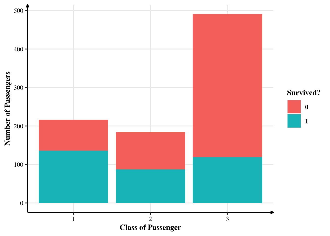
We can safely say that not many customers from class 3 survived.
Age of Passengers (and Survivors)
training %>%
   ggplot(aes(x = Age)) +
   geom_histogram(binwidth = 5)
## Warning: Removed 177 rows containing non-finite values (stat_bin).
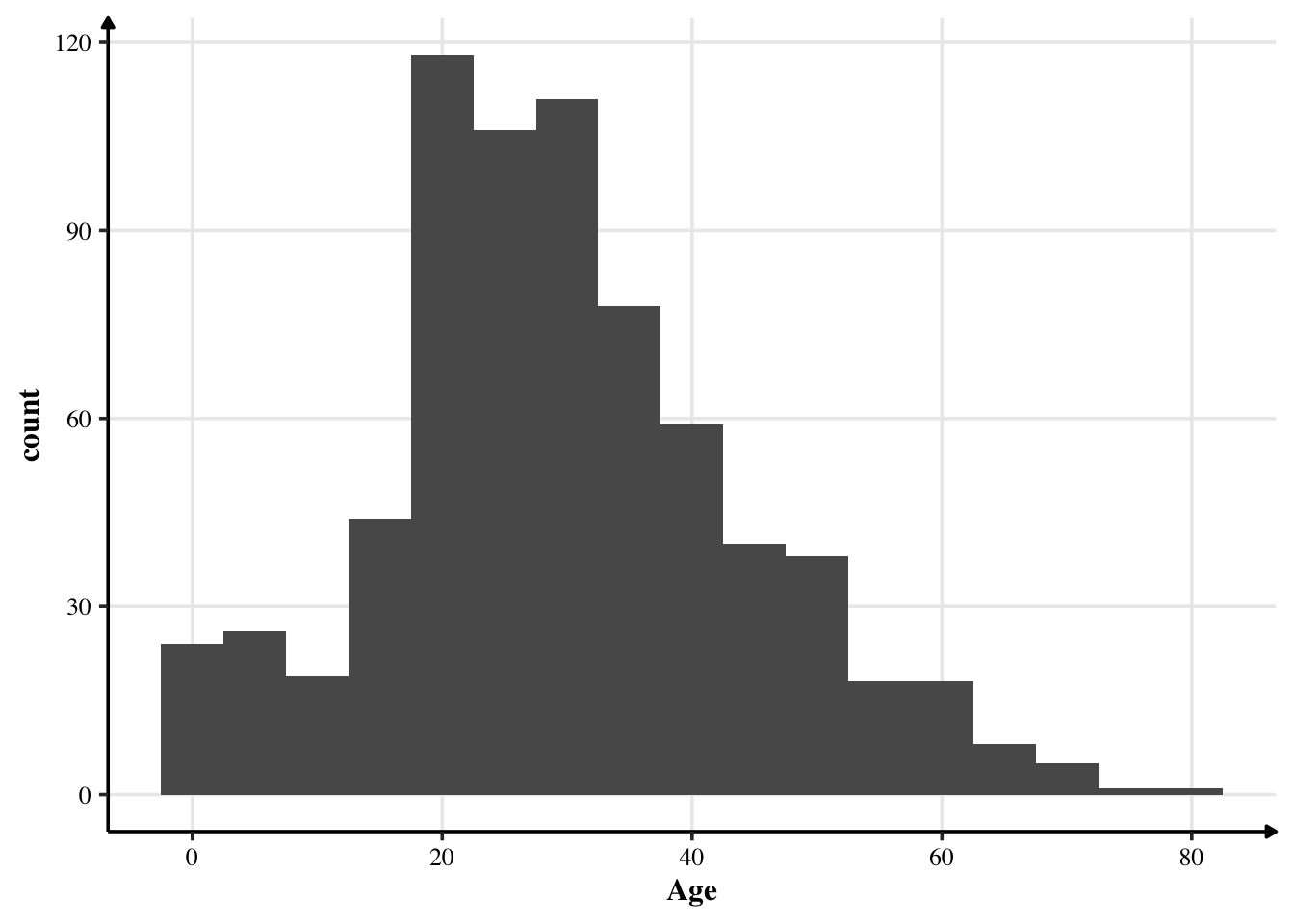
Most people were between the age of 20 and 40 years — so largely young people were travelling. At the same time, we also notice that the age is approximately normally distributed. Thus, we can impute the missing values with the mean.
Let’s see age-wise distribution of survival.
p = training %>%
   ggplot(aes(x = Age, fill = factor(Survived))) +
   geom_histogram(binwidth = 5) +
   labs(x = "Age of Passenger", y = "Number of Passengers",
        fill = "Survived?")

ggplotly(p)
## Warning: Removed 177 rows containing non-finite values (stat_bin).
So, younglings survived — those under 15 years of age. Probably this was because of the lifeguards’ instincts to save women and children first. (You can hover over the plot to know more.)
Number of Siblings/Spouses and Parents
training %>%
   count(SibSp) %>%
   ggplot(aes(x = SibSp, y = n)) +
   geom_col() +
   labs(x = "Number of Siblings", y = "Number of Passengers with `x` Siblings")
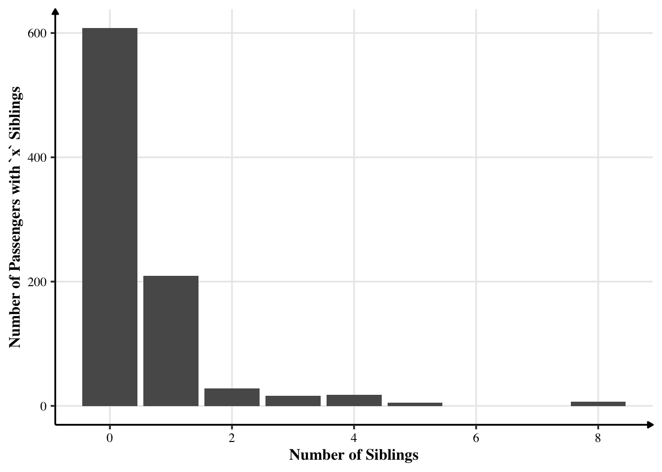
Most had no siblings. Some had one sibling or more siblings. Interestingly, no one had six or seven siblings.
training %>%
   count(Parch)
## # A tibble: 7 × 2
##   Parch     n
##   <dbl> <int>
## 1     0   678
## 2     1   118
## 3     2    80
## 4     3     5
## 5     4     4
## 6     5     5
## 7     6     1
training %>%
   count(Parch) %>%
   ggplot(aes(x = Parch, y = n)) +
   geom_col() +
   labs(x = "Number of Parents / Children", y = "Number of Passengers with `x` Parents / Children")
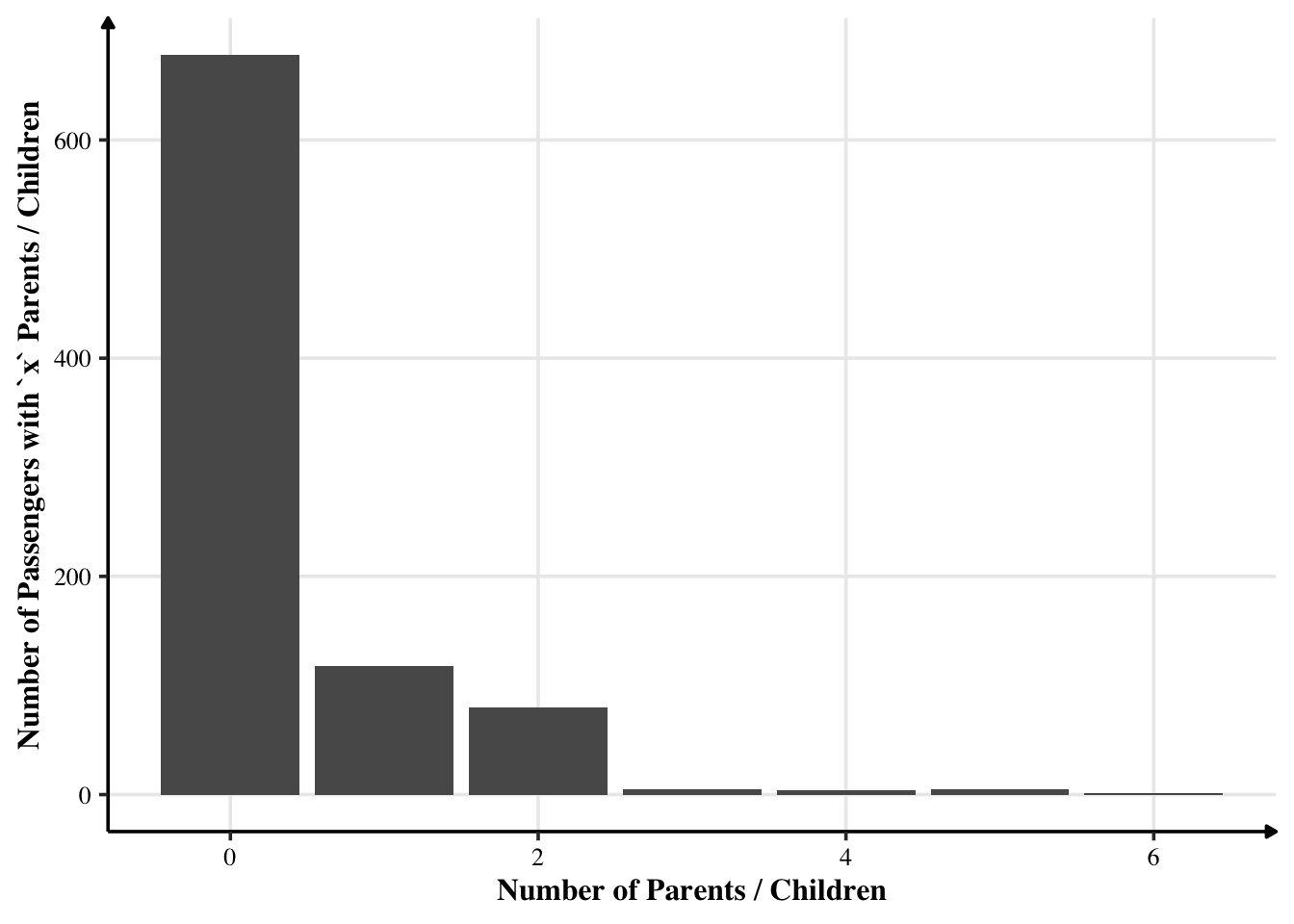
Most passengers were travelling alone. Some were travelling with 1 or 2 parents / children. Very few were travelling with their parents and children too.
Where did they Embark their Journey?
training %>%
   count(Embarked)
## # A tibble: 4 × 2
##   Embarked     n
##   <chr>    <int>
## 1 C          168
## 2 Q           77
## 3 S          644
## 4 <NA>         2
Most embarked their journey from Southampton. Cherbourg was the second most popular boarding point. Queenstown was the least popular one. There are two missing values that we can fill the mode. Let’s see them by grouping through survival.
training %>%
   count(Embarked, Survived)
## # A tibble: 7 × 3
##   Embarked Survived     n
##   <chr>       <dbl> <int>
## 1 C               0    75
## 2 C               1    93
## 3 Q               0    47
## 4 Q               1    30
## 5 S               0   427
## 6 S               1   217
## 7 <NA>            1     2
training %>%
   count(Embarked, Survived) %>%
   ggplot(aes(x = Embarked, y = n, fill = factor(Survived))) +
   geom_bar(position = "stack", stat="identity") +
   labs(x = "Boarding Point", y = "Number of Passengers",
        fill = "Survived?")
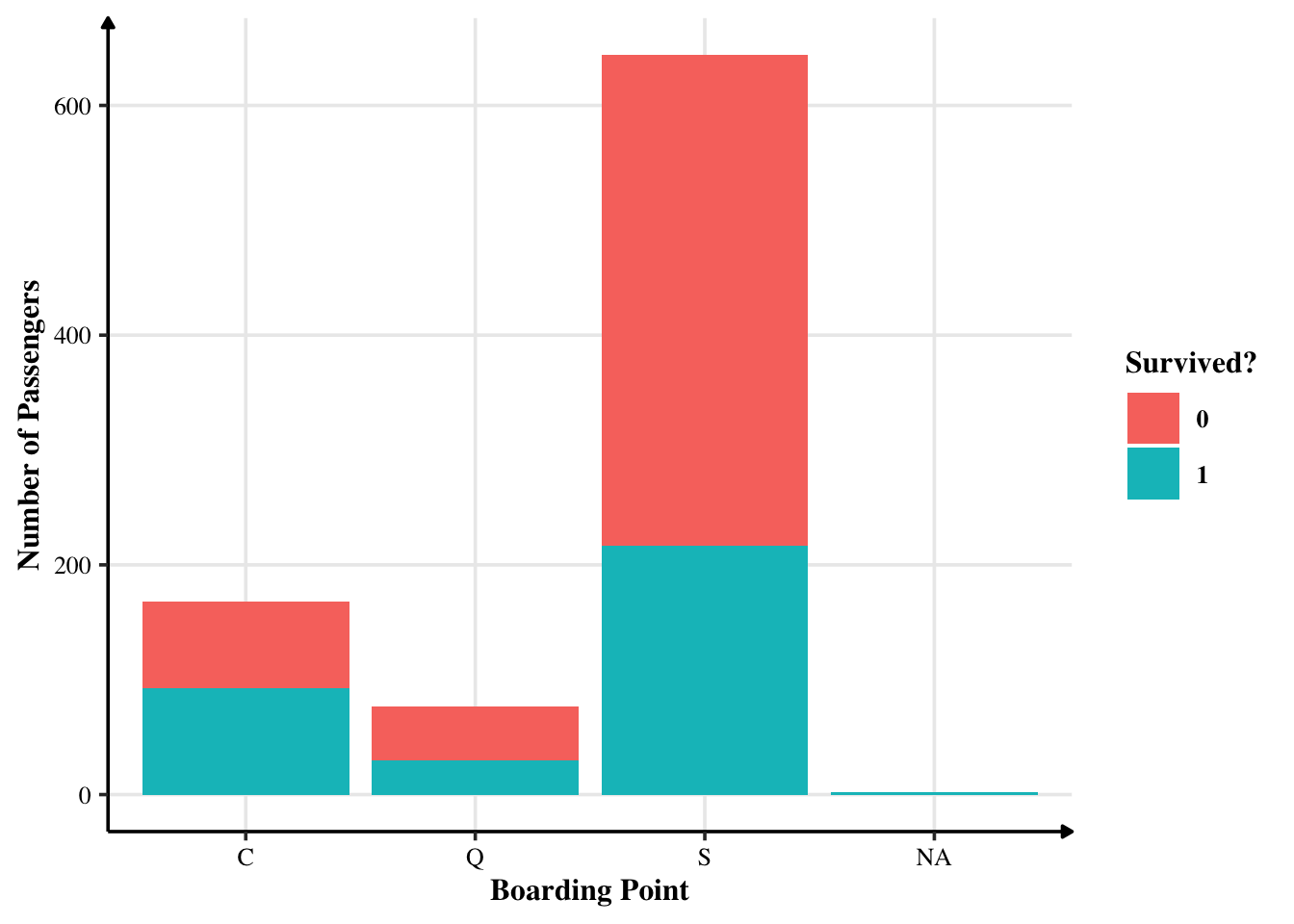
There seems to be little relationship between where they started their journey on whether they survived or not. Proportionally, there aren’t many changes.
Now, let’s start the cool part: machine learning.
Wrangling Data for Machine Learning
The dataset that we have is only one: training. The test one doesn’t have labels and the only way to check is to upload to Kaggle. I will do that at the end. Right now, I need to segregate my data into two sets: training and testing. By default, R does 75/25 split.
But first, I will remove Cabin — which is mostly missing.
set.seed(0)

training$Survived = factor(training$Survived)
training$Pclass = factor(training$Pclass)

training = training %>%
   select(-PassengerId, -Cabin, -Name, -Ticket)
split = initial_split(training, strata = Survived)

tit_train = training(split)
tit_test = testing(split)
Let’s Fill The Missing Values
How many values are missing right now in the training dataset?
sum(is.na(tit_train))
## [1] 137
There are a lot of missing values. Let’s see which variables are missing.
missing_df(tit_train)
## # A tibble: 8 × 2
##   names    miss_rate
##   <chr>        <dbl>
## 1 Survived   0
## 2 Pclass     0
## 3 Sex        0
## 4 Age        0.204
## 5 SibSp      0
## 6 Parch      0
## 7 Fare       0
## 8 Embarked   0.00150
Age and Embarked. As I had discussed earlier, I can fill them in with the mean and mode.
# Function for mode (borrowed from https://stackoverflow.com/questions/2547402/how-to-find-the-statistical-mode)
Mode = function(x) {
  ux = unique(x)
  ux[which.max(tabulate(match(x, ux)))]
}

mean_age = mean(tit_train$Age, na.rm = T)
mode_embark = Mode(tit_train$Embarked)
# Fill missing values with mean
fill_with_mean = function(x)
{
   x[is.na(x)] = mean(x, na.rm = T)
   return (x)
}

# Fill missing values with mode
fill_with_mode = function(x)
{
   x[is.na(x)] = Mode(x)
   return (x)
}
tit_train$Age = fill_with_mean(tit_train$Age)
tit_train$Embarked = fill_with_mode(tit_train$Embarked)
sum(is.na(tit_train))
## [1] 0
So, all missing values are gone!
Now, let’s do the same transformations to tit_test. Note that we will use training mean and mode for this purpose.
tit_test$Age[is.na(tit_test$Age)] = mean_age
tit_test$Embarked[is.na(tit_test$Embarked)] = mode_embark
sum(is.na(tit_test))
## [1] 0
Logistic Regression and xgboost Tree
The first method I want to try is generalised least squares, or logistic regression. Second I want to xgboost tree.
Note that our sample size is only 667. For most methods, this is very small. Thus, I will use bootstrapped samples.
tit_boot = bootstraps(tit_train, strata = Survived)
tit_boot
## # Bootstrap sampling using stratification
## # A tibble: 25 × 2
##    splits            id
##    <list>            <chr>
##  1 <split [667/246]> Bootstrap01
##  2 <split [667/244]> Bootstrap02
##  3 <split [667/249]> Bootstrap03
##  4 <split [667/242]> Bootstrap04
##  5 <split [667/231]> Bootstrap05
##  6 <split [667/239]> Bootstrap06
##  7 <split [667/257]> Bootstrap07
##  8 <split [667/230]> Bootstrap08
##  9 <split [667/238]> Bootstrap09
## 10 <split [667/249]> Bootstrap10
## # … with 15 more rows
So, this created 25 bootstrapped samples of different sizes.
Engine
Logistic Regression
# Specifying Recipe for converting nominal to binary
glm_rec = recipe(Survived ~ ., data = tit_train) %>%
   step_dummy(all_nominal_predictors())

# Logistic Regression
glm_spec = logistic_reg() %>%
   set_engine("glm")
xgboost Classification
# Specify Recipe
xg_rec = recipe(Survived ~ ., data = tit_train) %>%
  step_dummy(all_nominal_predictors())

# Specify Engine
xg_model = boost_tree(mode = "classification", # binary response
                       trees = tune(),
                       mtry = tune(),
                       tree_depth = tune(),
                       learn_rate = tune(),
                       loss_reduction = tune(),
                       min_n = tune()) # parameters to be tuned
Workflow
Logistic Regression
glm_wf = workflow() %>%
   add_model(glm_spec) %>%
   add_recipe(glm_rec)
xgboost Regression
The following cross-validation needs to be performed to choose the appropriate xgboost model.
cv_folds = vfold_cv(tit_train, v = 3, strata = Survived)
c_metrics = metric_set(accuracy, sens, roc_auc)

# Specify a baseline model control
control = control_resamples(save_pred = TRUE, verbose = F)

# Specify the workflow
xg_wf = workflow() %>%
  add_model(xg_model) %>%
  add_recipe(xg_rec)
Fitting the Models
Logistic Regression
Without bootstrapped samples:
glm_rs_unboot = glm_wf %>%
   fit(data = tit_train)
glm_rs_unboot
## ══ Workflow [trained] ══════════════════════════════════════════════════════════
## Preprocessor: Recipe
## Model: logistic_reg()
##
## ── Preprocessor ────────────────────────────────────────────────────────────────
## 1 Recipe Step
##
## • step_dummy()
##
## ── Model ───────────────────────────────────────────────────────────────────────
##
## Call:  stats::glm(formula = ..y ~ ., family = stats::binomial, data = data)
##
## Coefficients:
## (Intercept)          Age        SibSp        Parch         Fare    Pclass_X2
##   4.0983745   -0.0407578   -0.3150337   -0.0927634    0.0004301   -1.3108194
##   Pclass_X3     Sex_male   Embarked_Q   Embarked_S
##  -2.3795645   -2.7701258    0.3385133    0.0321918
##
## Degrees of Freedom: 666 Total (i.e. Null);  657 Residual
## Null Deviance:       888.3
## Residual Deviance: 592.1     AIC: 612.1
Let’s check its accuracy and confusion matrix.
predict(glm_rs_unboot, tit_train) %>%
   bind_cols(tit_train) %>%
   conf_mat(truth = Survived, estimate = .pred_class)
##           Truth
## Prediction   0   1
##          0 346  74
##          1  65 182
predict(glm_rs_unboot, tit_train) %>%
   bind_cols(tit_train) %>%
   accuracy(truth = Survived, estimate = .pred_class)
## # A tibble: 1 × 3
##   .metric  .estimator .estimate
##   <chr>    <chr>          <dbl>
## 1 accuracy binary         0.792
So, accuracy is 80.1%. This is a good accuracy. Let’s see AUC.
predict(glm_rs_unboot, tit_train, type = "prob") %>%
   bind_cols(tit_train) %>%
   roc_auc(.pred_0,truth = Survived)
## # A tibble: 1 × 3
##   .metric .estimator .estimate
##   <chr>   <chr>          <dbl>
## 1 roc_auc binary         0.856
0.843 as AUC score is not bad at all.
With bootstrapped samples:
glm_rs = glm_wf %>%
   fit_resamples(resamples = tit_boot,
                 control = control_resamples(save_pred = TRUE, verbose = F))
glm_rs
## # Resampling results
## # Bootstrap sampling using stratification
## # A tibble: 25 × 5
##    splits            id          .metrics         .notes           .predictions
##    <list>            <chr>       <list>           <list>           <list>
##  1 <split [667/246]> Bootstrap01 <tibble [2 × 4]> <tibble [0 × 1]> <tibble>
##  2 <split [667/244]> Bootstrap02 <tibble [2 × 4]> <tibble [0 × 1]> <tibble>
##  3 <split [667/249]> Bootstrap03 <tibble [2 × 4]> <tibble [0 × 1]> <tibble>
##  4 <split [667/242]> Bootstrap04 <tibble [2 × 4]> <tibble [0 × 1]> <tibble>
##  5 <split [667/231]> Bootstrap05 <tibble [2 × 4]> <tibble [0 × 1]> <tibble>
##  6 <split [667/239]> Bootstrap06 <tibble [2 × 4]> <tibble [0 × 1]> <tibble>
##  7 <split [667/257]> Bootstrap07 <tibble [2 × 4]> <tibble [0 × 1]> <tibble>
##  8 <split [667/230]> Bootstrap08 <tibble [2 × 4]> <tibble [0 × 1]> <tibble>
##  9 <split [667/238]> Bootstrap09 <tibble [2 × 4]> <tibble [0 × 1]> <tibble>
## 10 <split [667/249]> Bootstrap10 <tibble [2 × 4]> <tibble [0 × 1]> <tibble>
## # … with 15 more rows
glm_rs %>%
   collect_metrics()
## # A tibble: 2 × 6
##   .metric  .estimator  mean     n std_err .config
##   <chr>    <chr>      <dbl> <int>   <dbl> <chr>
## 1 accuracy binary     0.791    25 0.00413 Preprocessor1_Model1
## 2 roc_auc  binary     0.844    25 0.00455 Preprocessor1_Model1
Logistic regression with bootstrapped samples gives me an accuracy of 80.6% with AUC of 0.846. So, bootstrapping has reduced overfitting by a small amount.
Let’s see its ROC curve.
glm_rs %>%
   collect_predictions() %>%
   group_by(id) %>% # -- to get 25 ROC curves, for each bootstrapped sample
   roc_curve(Survived, .pred_0) %>%
   autoplot()
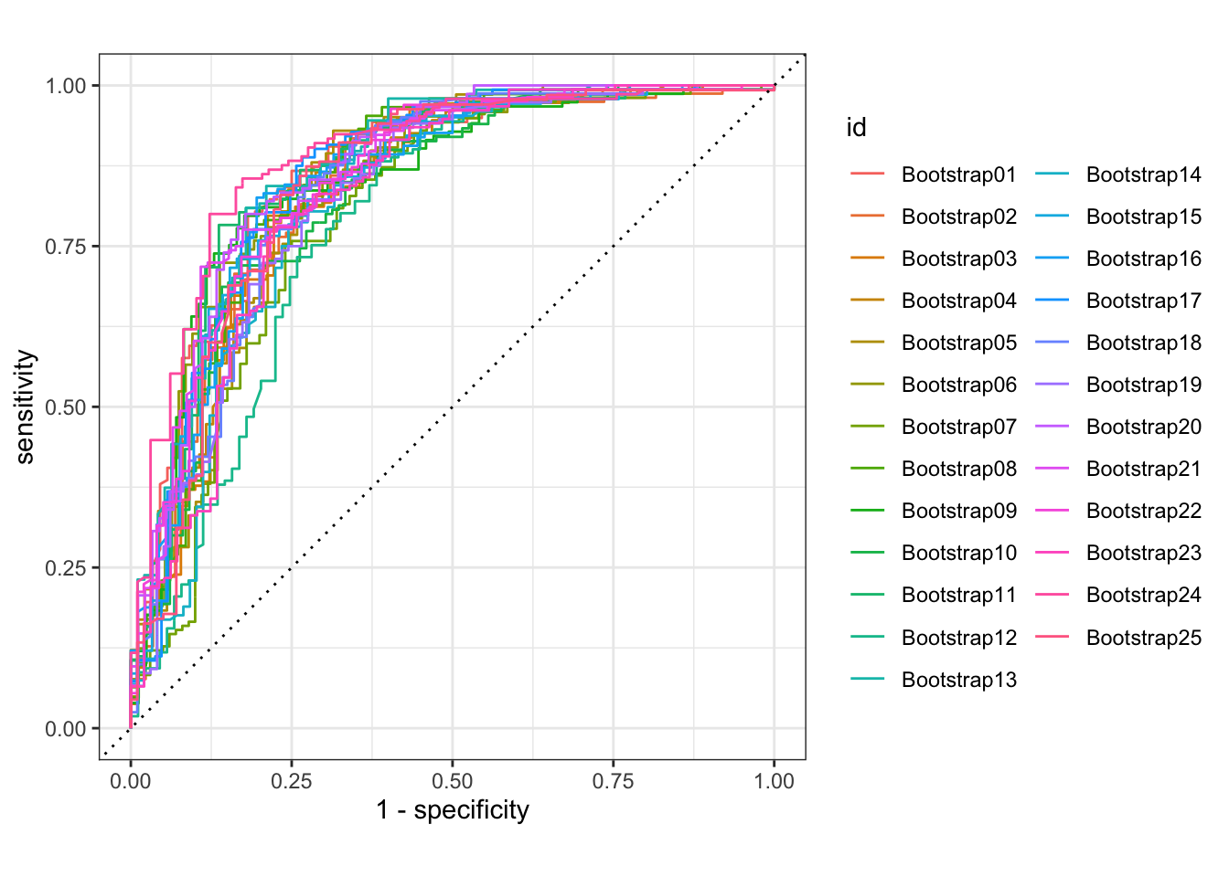
This is difficult to read so I will create a plot manually.
glm_rs %>%
   collect_predictions() %>%
   group_by(id) %>% # -- to get 25 ROC curves, for each bootstrapped sample
   roc_curve(Survived, .pred_0) %>%
   ggplot(aes(1 - specificity, sensitivity, col = id)) +
   geom_abline(lty = 2, colour = "grey80", size = 1.5) +
   geom_path(show.legend = FALSE, alpha = 0.5, size = 1.2) +
   coord_equal()
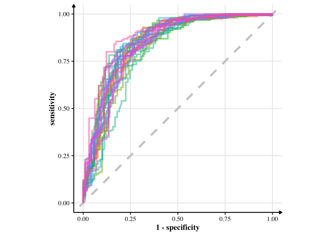
The model looks pretty good, if you ask me. Let’s create the final fit with all of training data.
# storing final glm model
glm_fit = glm_wf %>%
   fit(data = tit_train)
Check its metrics.
glm_fit %>%
   predict(tit_train) %>%
   bind_cols(tit_train) %>%
   conf_mat(truth = Survived, estimate = .pred_class)
##           Truth
## Prediction   0   1
##          0 346  74
##          1  65 182
glm_fit %>%
   predict(tit_train) %>%
   bind_cols(tit_train) %>%
   accuracy(truth = Survived, estimate = .pred_class)
## # A tibble: 1 × 3
##   .metric  .estimator .estimate
##   <chr>    <chr>          <dbl>
## 1 accuracy binary         0.792
glm_fit %>%
   predict(tit_train, type = "prob") %>%
   bind_cols(tit_train) %>%
   roc_auc(truth = Survived, estimate = .pred_0)
## # A tibble: 1 × 3
##   .metric .estimator .estimate
##   <chr>   <chr>          <dbl>
## 1 roc_auc binary         0.856
xgboost Model
xg_tune = xg_wf %>%
  tune_grid(cv_folds,
            metrics = c_metrics,
            control = control,
            grid = crossing(trees = 1000,
                            mtry = c(3, 5, 8),
                            tree_depth = c(5, 10, 15),
                            learn_rate = c(0.01, 0.005),
                            loss_reduction = c(0.01, 0.1, 1),
                            min_n = c(2, 10, 25)))
I’m manually specifying grid values to try. Let’s visualise the models.
autoplot(xg_tune)
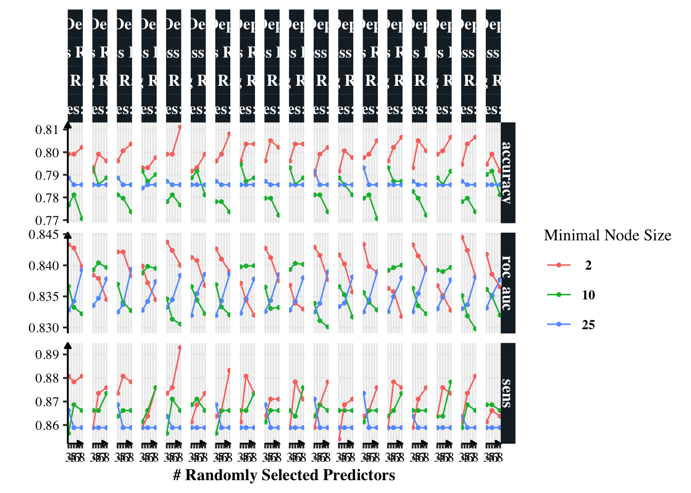
Having minimal node size as two gives a minor benefit in accuracy. Other than that, I am confused to know which model is the best. Thus, I will use show_best() to find the best model.
show_best(xg_tune, metric = "roc_auc")
## # A tibble: 5 × 12
##    mtry trees min_n tree_depth learn_rate loss_reduction .metric .estimator
##   <dbl> <dbl> <dbl>      <dbl>      <dbl>          <dbl> <chr>   <chr>
## 1     3  1000     2         15      0.005           1    roc_auc binary
## 2     3  1000     2          5      0.005           1    roc_auc binary
## 3     3  1000     2         15      0.005           0.01 roc_auc binary
## 4     3  1000     2          5      0.005           0.01 roc_auc binary
## 5     3  1000     2         15      0.005           0.1  roc_auc binary
## # … with 4 more variables: mean <dbl>, n <int>, std_err <dbl>, .config <chr>
show_best(xg_tune, metric = "accuracy")
## # A tibble: 5 × 12
##    mtry trees min_n tree_depth learn_rate loss_reduction .metric  .estimator
##   <dbl> <dbl> <dbl>      <dbl>      <dbl>          <dbl> <chr>    <chr>
## 1     8  1000     2          5      0.005           1    accuracy binary
## 2     8  1000     2         10      0.005           0.01 accuracy binary
## 3     8  1000     2         15      0.005           1    accuracy binary
## 4     8  1000     2         15      0.01            0.01 accuracy binary
## 5     8  1000     2         15      0.01            0.1  accuracy binary
## # … with 4 more variables: mean <dbl>, n <int>, std_err <dbl>, .config <chr>
The best model has an accuracy of 0.822 and AUC of 0.861. The good news is that both give me the same model (i.e. have the same hyper-parameters). Thus, I am at a good place.
best_model = select_best(xg_tune, metric = "roc_auc")
Let’s finalise the model and train it on all of training set.
xg_fit = xg_wf %>%
   finalize_workflow(best_model) %>%
   fit(data = tit_train)
## [15:15:10] WARNING: amalgamation/../src/learner.cc:1115: Starting in XGBoost 1.3.0, the default evaluation metric used with the objective 'binary:logistic' was changed from 'error' to 'logloss'. Explicitly set eval_metric if you'd like to restore the old behavior.
xg_fit
## ══ Workflow [trained] ══════════════════════════════════════════════════════════
## Preprocessor: Recipe
## Model: boost_tree()
##
## ── Preprocessor ────────────────────────────────────────────────────────────────
## 1 Recipe Step
##
## • step_dummy()
##
## ── Model ───────────────────────────────────────────────────────────────────────
## ##### xgb.Booster
## raw: 3 Mb
## call:
##   xgboost::xgb.train(params = list(eta = 0.005, max_depth = 15,
##     gamma = 1, colsample_bytree = 1, colsample_bynode = 0.333333333333333,
##     min_child_weight = 2, subsample = 1, objective = "binary:logistic"),
##     data = x$data, nrounds = 1000, watchlist = x$watchlist, verbose = 0,
##     nthread = 1)
## params (as set within xgb.train):
##   eta = "0.005", max_depth = "15", gamma = "1", colsample_bytree = "1", colsample_bynode = "0.333333333333333", min_child_weight = "2", subsample = "1", objective = "binary:logistic", nthread = "1", validate_parameters = "TRUE"
## xgb.attributes:
##   niter
## callbacks:
##   cb.evaluation.log()
## # of features: 9
## niter: 1000
## nfeatures : 9
## evaluation_log:
##     iter training_logloss
##        1         0.690979
##        2         0.689212
## ---
##      999         0.304644
##     1000         0.304552
Checking its confusion matrix, accuracy and other metrics.
predict(xg_fit, tit_train) %>%
   bind_cols(tit_train) %>%
   conf_mat(truth = Survived, estimate = .pred_class)
##           Truth
## Prediction   0   1
##          0 389  50
##          1  22 206
predict(xg_fit, tit_train) %>%
   bind_cols(tit_train) %>%
   accuracy(truth = Survived, estimate = .pred_class)
## # A tibble: 1 × 3
##   .metric  .estimator .estimate
##   <chr>    <chr>          <dbl>
## 1 accuracy binary         0.892
predict(xg_fit, tit_train, type = "prob") %>%
   bind_cols(tit_train) %>%
   roc_auc(truth = Survived, estimate = .pred_0)
## # A tibble: 1 × 3
##   .metric .estimator .estimate
##   <chr>   <chr>          <dbl>
## 1 roc_auc binary         0.946
So, this final model has 89.2% accuracy with 0.939 after being trained on all of data.
Let’s look at the important predictors according to it.
importances = xgboost::xgb.importance(model = extract_fit_engine(xg_fit))
importances %>%
  mutate(Feature = fct_reorder(Feature, Gain)) %>%
  ggplot(aes(Gain, Feature)) +
  geom_col()
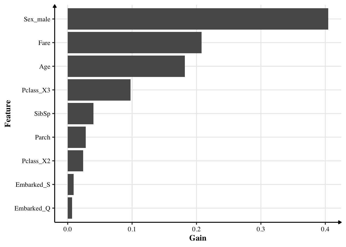
Being a male had actually a significant effect in surviving. Fare — which likely represents which class people were from — also can tell us will they survive. Passengers in class 3 are the most important result. I had expected people from class 1 (upper class) are more likely to survive than those from lower class. However, the opposite is true. Where they embarked from has little effect.
Comparing Logistic Regression and xgboost (Training Sets)
| Model | Accuracy | ROC Area Under Curve |
|---|---|---|
| Logistic Regression | 0.792 | 0.856 |
| Logistic Regression (with Bootstrapped Samples) | 0.792 | 0.856 |
| xgboost | 0.894 | 0.951 |
Accuracy and AUC for Logistic Regression and xgboost
Boosted regression trees perform better than logistic regression, around 10 per cent better. Let’s test both models on test dataset.
Testing Model
Let’s test the models on tit_test.
Logistic Regression (with Bootstraps)
glm_fit %>%
   predict(tit_test) %>%
   bind_cols(tit_test) %>%
   conf_mat(truth = Survived, estimate = .pred_class)
##           Truth
## Prediction   0   1
##          0 113  22
##          1  25  64
glm_fit %>%
   predict(tit_test) %>%
   bind_cols(tit_test) %>%
   accuracy(truth = Survived, estimate = .pred_class)
## # A tibble: 1 × 3
##   .metric  .estimator .estimate
##   <chr>    <chr>          <dbl>
## 1 accuracy binary         0.790
glm_fit %>%
   predict(tit_test, type = "prob") %>%
   bind_cols(tit_test) %>%
   roc_auc(truth = Survived, estimate = .pred_0)
## # A tibble: 1 × 3
##   .metric .estimator .estimate
##   <chr>   <chr>          <dbl>
## 1 roc_auc binary         0.850
xgboost
predict(xg_fit, tit_test) %>%
   bind_cols(tit_test) %>%
   conf_mat(truth = Survived, estimate = .pred_class)
##           Truth
## Prediction   0   1
##          0 120  19
##          1  18  67
predict(xg_fit, tit_test) %>%
   bind_cols(tit_test) %>%
   accuracy(truth = Survived, estimate = .pred_class)
## # A tibble: 1 × 3
##   .metric  .estimator .estimate
##   <chr>    <chr>          <dbl>
## 1 accuracy binary         0.835
predict(xg_fit, tit_test, type = "prob") %>%
   bind_cols(tit_test) %>%
   roc_auc(truth = Survived, estimate = .pred_0)
## # A tibble: 1 × 3
##   .metric .estimator .estimate
##   <chr>   <chr>          <dbl>
## 1 roc_auc binary         0.881
| Model | Accuracy | ROC Area under Curve |
|---|---|---|
| Logistic Regression (Bootstrapped) | 0.790 | 0.850 |
| xgboost | 0.830 | 0.884 |
Test accuracies for logistic regression and xgboost model.
xgboost model performs a little better. Since Kaggle judges only by accuracy (and I’d argue the task of machine learning is to predict with little focus on inference), I would consider xgboost for the final model.