Stackoverflow Answers
Most of the time when I answer questions on Stack Overflow, I end up learning a thing or two about R myself. Answering questions gets me warmed up on unrelated topics. These questions are one of their kind. This blog post documents all my answers so that I can find the answers readily.
The headlines explain the basic logic of what I am trying to achieve through that question.
Visualisation
This question was on combining time series plots using par().
par() won’t work because plot.decomposed.ts() (which we implicitly call when calling plot()) isn’t designed to work that way. The most straightforward alternative is to use autoplot() from the forecast package to generate decomposition plots and combine them using patchwork.
Here is an example.
# Loading forecast and patchwork
library(forecast)
## Registered S3 method overwritten by 'quantmod':
## method from
## as.zoo.data.frame zoolibrary(patchwork)
m1 = decompose(co2)
m2 = decompose(AirPassengers)
m3 = decompose(UKgas)
p1 = autoplot(m1)
p2 = autoplot(m2)
p3 = autoplot(m3)
p1 / p2 / p3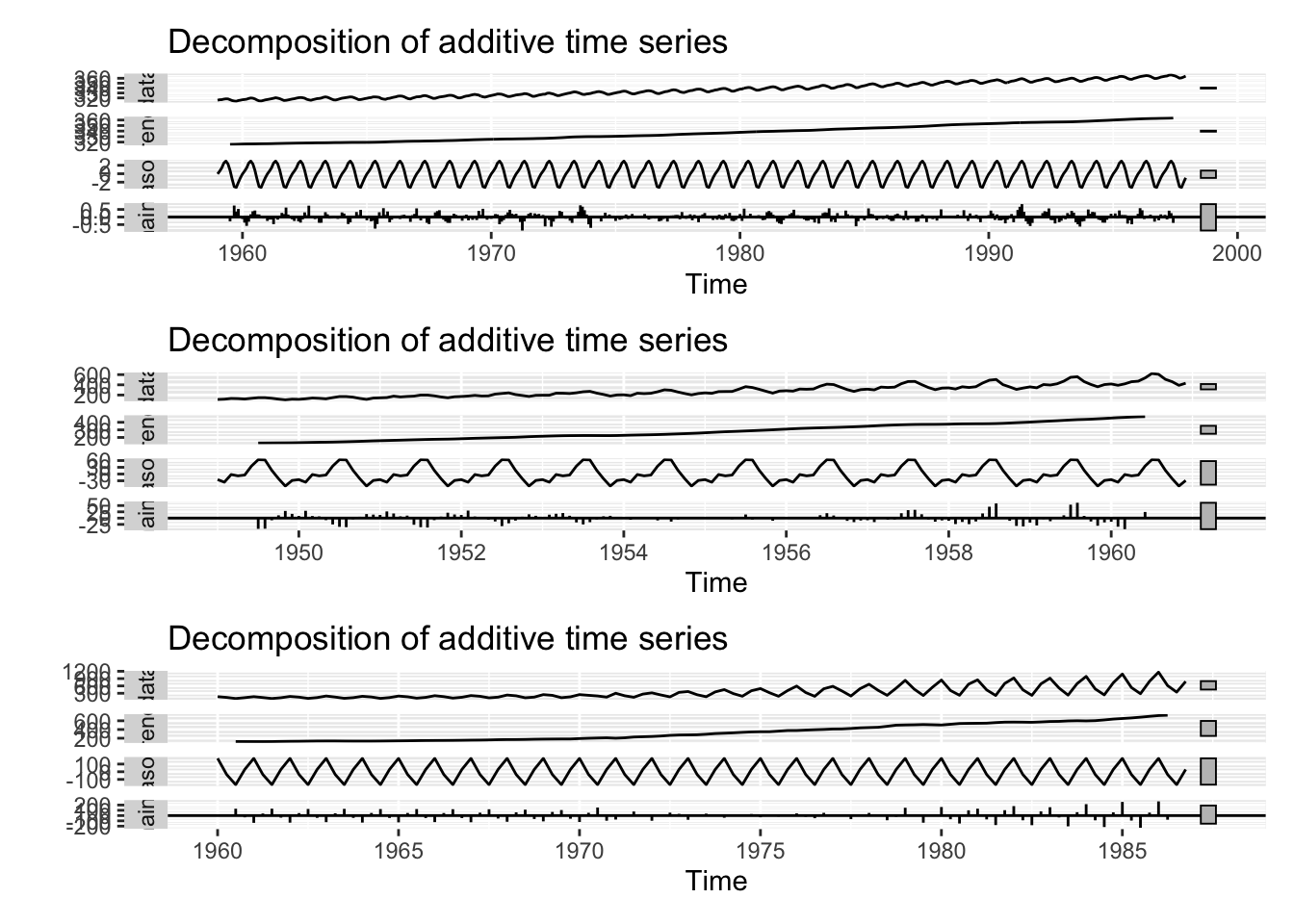
The last line, p1 / p2 / p3, tells R to stack them vertically. If you want to stack them horizontally, use p1 + p2 + p3. If you’re being feisty, you can also try (p1 + p2)/p3 to stack the first two horizontally and the last one beneath it.
Using gghighlight to highlight a line plot in ggplot2
gghighlight provides gghighlight() which can be used to selectively highlight some lines, points or other geom_. I couldn’t get the dataset in question working, so I generated a random dataset. The code should work for their case as well.
library(gghighlight)## Loading required package: ggplot2year = 1970:2020
value = rnorm(length(year), 2000, 5)
x = c("A", "B", "C", "D", "E")
variable = sample(x, length(year), replace = T)
df = data.frame(year = year,
value = value,
variable = variable)Now is the cool part.
df %>%
  ggplot(aes(x = year, y = value, colour = variable)) +
  geom_line() +
  gghighlight(variable == "A") +
  theme_minimal()
## Warning: Tried to calculate with group_by(), but the calculation failed.
## Falling back to ungrouped filter operation...## label_key: variable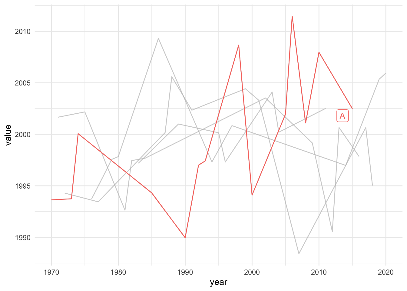
Voila!
Histogram with ggplot2
I had to clarify several things. First, what made them choose bins = 43? Second, is providing the scale manually necessary? If the data is in the right format, they should not need it. If it isn’t, they should first transform the data and then do it.
Third, gray background (which they wanted to change) is from the default theme. There are several options but I like minimal. minimal, linedraw and bw have white grids.
(I’m generating 1000 random numbers for this example.)
library(tidyverse)## ── Attaching core tidyverse packages ──────────────────────── tidyverse 2.0.0 ──
## ✔ dplyr 1.1.2 ✔ readr 2.1.4
## ✔ forcats 1.0.0 ✔ stringr 1.5.0
## ✔ lubridate 1.9.2 ✔ tibble 3.2.1
## ✔ purrr 1.0.2 ✔ tidyr 1.3.0
## ── Conflicts ────────────────────────────────────────── tidyverse_conflicts() ──
## ✖ dplyr::filter() masks stats::filter()
## ✖ dplyr::lag() masks stats::lag()
## ℹ Use the conflicted package (<http://conflicted.r-lib.org/>) to force all conflicts to become errorsv = tibble(var = rnorm(1000))
ggplot(v, aes(x = var)) +
geom_histogram(bins = 20) +
theme_minimal()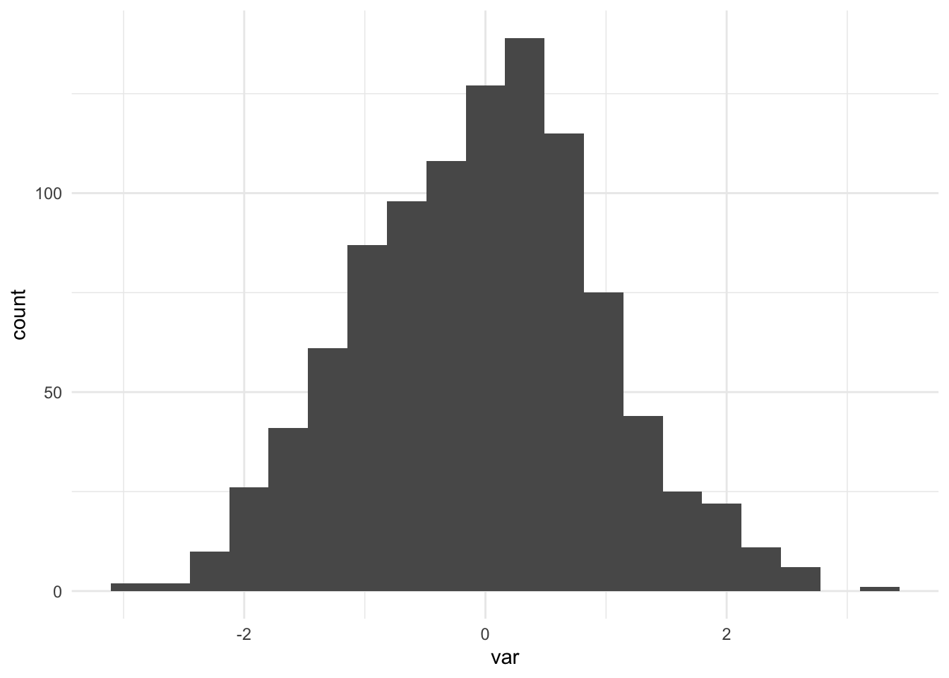
Barplots grouped by two (factor) variables and plotting mean values as points on them
The data they posted didn’t work so I’ve used (modified) iris dataset.
# loading tidyverse
library(tidyverse)

# adding another factor variable to replicate this example
iris$Variable = rep(LETTERS[1:5], times = 30)
Here’s the meat.
iris %>%
  ggplot(aes(x = Species, y = Sepal.Length, fill = Variable)) +
  geom_boxplot() +
  stat_summary(
    fun = mean,
    color = "steelblue",
    position = position_dodge(0.75),
    geom = "point",
    shape = 20,
    size = 5,
    show.legend = FALSE
  ) +
  theme_minimal()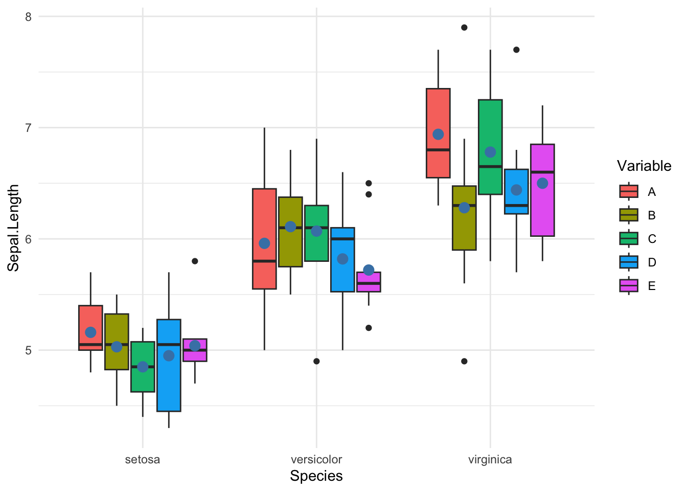
String Manipulations
Selecting rows where a string match occurs
We can use grepl() from base R for this. grepl() returns True if the word is present and False otherwise.
text = "The Little Vanities of Mrs. Whittaker: A Novel"
word = "Novel"

grepl(word, text)
## [1] TRUEThe original_books file (in question) will require large downloads so I’m showing an example of searching “Plays” in title.x of their novels data frame.
library(gutenbergr)
library(tidyverse)

gutenberg_full_data <-
  left_join(gutenberg_works(language == "en"), gutenberg_metadata, by = "gutenberg_id")

gutenberg_full_data <-
  left_join(gutenberg_full_data, gutenberg_subjects)
## Joining with `by = join_by(gutenberg_id)`gutenberg_full_data <-
subset(
gutenberg_full_data,
select = -c(
rights.x,
has_text.x,
language.y,
gutenberg_bookshelf.x,
gutenberg_bookshelf.y,
rights.y,
has_text.y,
gutenberg_bookshelf.y,
gutenberg_author_id.y,
title.y,
author.y
)
)
gutenberg_full_data <-
gutenberg_full_data[-which(is.na(gutenberg_full_data$author.x)), ]
novels <- gutenberg_full_data %>% filter(subject == "Drama")Here comes the cool part.
novels %>%
  mutate(contains_play = grepl("Plays", title.x)) %>%
  as.data.frame() %>%
  head()
## gutenberg_id title.x
## 1 1308 A Florentine Tragedy; La Sainte Courtisane
## 2 2270 Shakespeare's First Folio
## 3 2587 Life Is a Dream
## 4 4970 There Are Crimes and Crimes
## 5 5053 Plays by August Strindberg: Creditors. Pariah.
## 6 5618 Six Plays
## author.x gutenberg_author_id.x language.x
## 1 Wilde, Oscar 111 en
## 2 Shakespeare, William 65 en
## 3 Calderón de la Barca, Pedro 970 en
## 4 Strindberg, August 1609 en
## 5 Strindberg, August 1609 en
## 6 Darwin, Florence Henrietta Fisher, Lady 1814 en
## subject_type subject contains_play
## 1 lcsh Drama FALSE
## 2 lcsh Drama FALSE
## 3 lcsh Drama FALSE
## 4 lcsh Drama FALSE
## 5 lcsh Drama TRUE
## 6 lcsh Drama TRUENote that grepl() allows the second argument to be a vector. Thus, using rowwise() is not necessary. If it allowed searching only within a string, we would have to use rowwise().
Data Wrangling and Manipulation
Typecasting to Numeric
The variable born is registered as a character variable. Convert it to numeric and one should be good to go.
dat1$born = as.numeric(dat1$born)Now compute the age difference.
Grabbing columns from one data frame with variable names from another data frame
One can do it using any_of() function from dplyr. It selects the variables which match the names and ignores those which do not. I will use a list to store matrices from the loop. They can be accessed using df_modified[[i]].
df1=data.frame(q1 = c(1:3),
               q2 = c("One" , "Two" , "Three") ,
               q3 = c(100,231,523),
               q4 = c("red", "green", "blue"),
               q1.2 = c(20:22),
               q2.2 = c("Six" , "Ten" , "Twenty") ,
               q3.2 = c(5,900,121),
               q4.2 = c("purple", "yellow", "white"))
df2=data.frame(x1 = c("q1" , "q2.1" , "q3.2" , "q4.2") ,
               x2 = c("q2" , "q3" , "q3.3" , "q4.4") ,
               x3 = c("q3" , "q2.4" , "q3.3" , "q4.6"),
               x4 = c("q4" , "q3.6" , "q3.3" , "q4.2"))
# Loading libraries
library(tidyverse)
df_modified = list()
for(i in 1:nrow(df2))
{
vars = as.character(df2[i,])
df_modified[[i]] = df1 %>%
select(any_of(vars))
}Output
df_modified## [[1]]
## q1 q2 q3 q4
## 1 1 One 100 red
## 2 2 Two 231 green
## 3 3 Three 523 blue
##
## [[2]]
## q3
## 1 100
## 2 231
## 3 523
##
## [[3]]
## q3.2
## 1 5
## 2 900
## 3 121
##
## [[4]]
## q4.2
## 1 purple
## 2 yellow
## 3 whiteDone!
Selecting Observations by Filtering Other Variables
One approach is to write a function that does that for you. It matches the first three variables with what you input and returns the index(or indexes) of elements that match.
which() returns the index of items that satisfy the condition. When I say which(df[,1] == a), it will return me the index of observations in df where the first column matches a. And so on. Then, you can use intersect() to find the common indexes in x1, x2 and x3. I’m using magrittr pipes %>% to simplify the coding.
check_this = function(df, a, b, c)
{
  x1 = which(df[,1] == a)
  x2 = which(df[,2] == b)
  x3 = which(df[,3] == c)

  v = intersect(x1, x2) %>%
    intersect(x3)
  return(v)
}
Minimum Working Example First, I’ll create a dummy data frame. Then, I’ll find the index using the function I just created.
df = tibble(var1 = 1:10,
            var2 = 11:20,
            var3 = letters[1:10],
            var4 = LETTERS[1:10])

df
## # A tibble: 10 × 4
## var1 var2 var3 var4
## <int> <int> <chr> <chr>
## 1 1 11 a A
## 2 2 12 b B
## 3 3 13 c C
## 4 4 14 d D
## 5 5 15 e E
## 6 6 16 f F
## 7 7 17 g G
## 8 8 18 h H
## 9 9 19 i I
## 10 10 20 j JNow, let us see it in action. First, I’ll pass the data frame and variables I want to match as arguments. The function will return the indices which I’ll store in l. Then, I’ll ask R to show me the rows which have indices numbers in l.
# checking and storing the index of matched
l = check_this(df, 2, 12, "b")

df[l,]
## # A tibble: 1 × 4
## var1 var2 var3 var4
## <int> <int> <chr> <chr>
## 1 2 12 b BNote: You could have skipped the step of storing indices in l by returning the selected rows of the data frame itself. The function would change to the following.
# the function
check_this = function(df, a, b, c)
{
  x1 = which(df[,1] == a)
  x2 = which(df[,2] == b)
  x3 = which(df[,3] == c)

  v = intersect(x1, x2) %>%
    intersect(x3)
  return(df[v,])
}
Convert a vector of strings in multiple formats into dates in R
My Solution
# sample date
dates <- c("2015-02-23","2015-02-12","2015-18-02","2015-25-02")

# libraries
library(testit) #for has_warning
library(lubridate) #for date functions
This function will correct the dates.
correct_dates = function(dates)
{
  dates_new = character()
  for(i in 1:length(dates))
  {
    #print(i)
    if(has_warning(day(ydm(dates[i]))>12))
      {dates_new = append(dates_new, ymd(dates[i]))}
    else
      {dates_new = append(dates_new, ydm(dates[i]))}
  }
  return(dates_new)
}
Let’s see it in action.
dates## [1] "2015-02-23" "2015-02-12" "2015-18-02" "2015-25-02"correct_dates(dates)## [1] "2015-02-23" "2015-12-02" "2015-02-18" "2015-02-25"Much Better Solution
dates <- c("2017-12-31","2017-12-30","2017-29-12","2017-28-12")
as.Date(lubridate::parse_date_time(dates, c('ymd', 'ydm')))
## [1] "2017-12-31" "2017-12-30" "2017-12-29" "2017-12-28"Table Formatting in kableExtra
How to append two tables with same number of columns in kableExtra?
I don’t know how to combine the tables directly without first joining the data frames. However, using pack_rows to specify rows for grouping together should work for this purpose.
library(kableExtra)##
## Attaching package: 'kableExtra'## The following object is masked from 'package:dplyr':
##
## group_rowsdf1 = data.frame(x = c("a","b"), y=1:2)
df2 = data.frame(x = c("c","d"), y=3:4)
rbind(df1, df2) %>%
kbl(format = "latex", caption = "Combined Tables") %>%
kable_paper("striped", full_width = F) %>%
pack_rows("Header 1", 1, 2) %>%
pack_rows("Header 2", 3, 4)Check the documentation of ?pack_rows from kableExtra to modify the group labels, add \hlines, or other such cosmetic changes.

Simulation
How many people are needed such that there is at least a 70% chance that one of them is born on the last day of December?
The question is, “How many people are needed such that there is at least a 70% chance that one of them is born on the last day of December?”. What they were finding now is “How many people are needed such that 70% have their birthdays on the last day of December?”. The answer to the second question is close to zero. But the first one is much simpler.
Replacing prob <- length(which(birthday == 365)) / people with check = any(birthday == 365) in their logic because at least one of them has to be born on Dec 31 will work. Then, they will be able to find if that number of people will have at least one person born on Dec 31.
After that, they will have to rerun the simulation multiple times to generate empirical probability distribution (kind of Monte Carlo). Only then they can check for probability.
Simulation Code
people_count = function(i)
{
  set.seed(i)
  for (people in 1:10000)
  {
    birthday = sample(365, size = people, replace = TRUE)
    check = any(birthday == 365)
    if(check == TRUE)
    {
      pf = people
      break
    }
  }
  return(pf)
}
people_count() function returns the number of people required to have so that at least one of them was born on Dec 31. Then I rerun the simulation 10,000 times.
# Number of simulations
nsim = 10000
l = lapply(1:nsim, people_count) %>%
  unlist()
Let’s see the distribution of the number of people required.
hist(l, main = "Histogram of # People",
     xlab = "# People")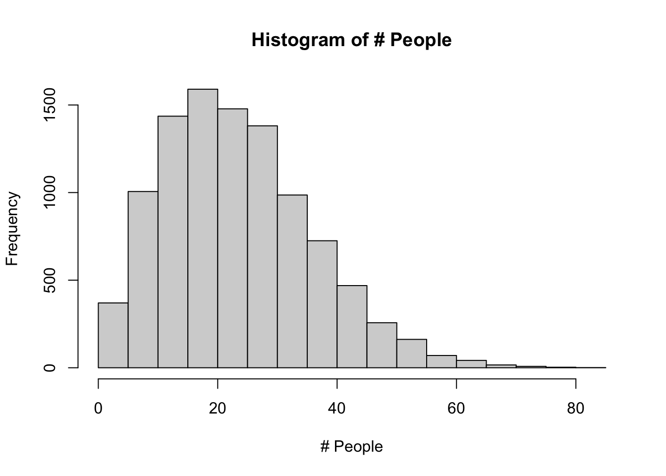
To find actual probability, I’ll use cumsum().
cdf = cumsum(l/nsim)
which(cdf>0.7)[1]
## [1] 292So, on average, you would need 292 people to have more than a 70% chance.