Classification: Logistic Regression and Random Forest
In this tutorial-cum-note, I will demonstrate how to use Logistic Regression and Random Forest algorithms to predict sex of a penguin. The data penguins comes from palmerpenguins package in R. It was collected by Dr. Kristen Gorman on three species of penguins at the Palmer Station, Antarctica LTER, a member of the Long Term Ecological Research Network.
The goal is to build a classifier model that predicts sex of the penguins given its physical characteristics.
The dataset can be installed from CRAN.
# If you don't have palmerpenguins package, first install it.
# install.packages("palmerpenguins")

# Loading Libraries
library(tidyverse)
## ── Attaching core tidyverse packages ──────────────────────── tidyverse 2.0.0 ──
## ✔ dplyr 1.1.2 ✔ readr 2.1.4
## ✔ forcats 1.0.0 ✔ stringr 1.5.0
## ✔ ggplot2 3.4.3 ✔ tibble 3.2.1
## ✔ lubridate 1.9.2 ✔ tidyr 1.3.0
## ✔ purrr 1.0.2
## ── Conflicts ────────────────────────────────────────── tidyverse_conflicts() ──
## ✖ dplyr::filter() masks stats::filter()
## ✖ dplyr::lag() masks stats::lag()
## ℹ Use the conflicted package (<http://conflicted.r-lib.org/>) to force all conflicts to become errorslibrary(palmerpenguins)
# setting my personal theme
theme_set(theme_h())
# Loading data
data("penguins")
penguins## # A tibble: 344 × 8
## species island bill_length_mm bill_depth_mm flipper_length_mm body_mass_g
## <fct> <fct> <dbl> <dbl> <int> <int>
## 1 Adelie Torgersen 39.1 18.7 181 3750
## 2 Adelie Torgersen 39.5 17.4 186 3800
## 3 Adelie Torgersen 40.3 18 195 3250
## 4 Adelie Torgersen NA NA NA NA
## 5 Adelie Torgersen 36.7 19.3 193 3450
## 6 Adelie Torgersen 39.3 20.6 190 3650
## 7 Adelie Torgersen 38.9 17.8 181 3625
## 8 Adelie Torgersen 39.2 19.6 195 4675
## 9 Adelie Torgersen 34.1 18.1 193 3475
## 10 Adelie Torgersen 42 20.2 190 4250
## # ℹ 334 more rows
## # ℹ 2 more variables: sex <fct>, year <int>We see that there are many missing instances. Let’s see how many of them are missing.
sum(is.na(penguins))## [1] 19So, nineteen entries are missing. Most likely, I will exclude them from the analysis at present but before that, I want to explore the data as it is.
Exploration
One of the best methods to do it is via count() from dplyr.
penguins %>%
   count(species)
## # A tibble: 3 × 2
## species n
## <fct> <int>
## 1 Adelie 152
## 2 Chinstrap 68
## 3 Gentoo 124penguins %>%
count(island)## # A tibble: 3 × 2
## island n
## <fct> <int>
## 1 Biscoe 168
## 2 Dream 124
## 3 Torgersen 52penguins %>%
count(species, island)## # A tibble: 5 × 3
## species island n
## <fct> <fct> <int>
## 1 Adelie Biscoe 44
## 2 Adelie Dream 56
## 3 Adelie Torgersen 52
## 4 Chinstrap Dream 68
## 5 Gentoo Biscoe 124penguins %>%
count(sex)## # A tibble: 3 × 2
## sex n
## <fct> <int>
## 1 female 165
## 2 male 168
## 3 <NA> 11penguins %>%
count(year)## # A tibble: 3 × 2
## year n
## <int> <int>
## 1 2007 110
## 2 2008 114
## 3 2009 120Cool. It looks pretty balanced.
penguins %>%
   filter(!is.na(sex)) %>%
   ggplot(aes(flipper_length_mm, bill_length_mm, colour = sex, size = body_mass_g)) +
   geom_point(alpha = 0.6) +
   facet_wrap(~species)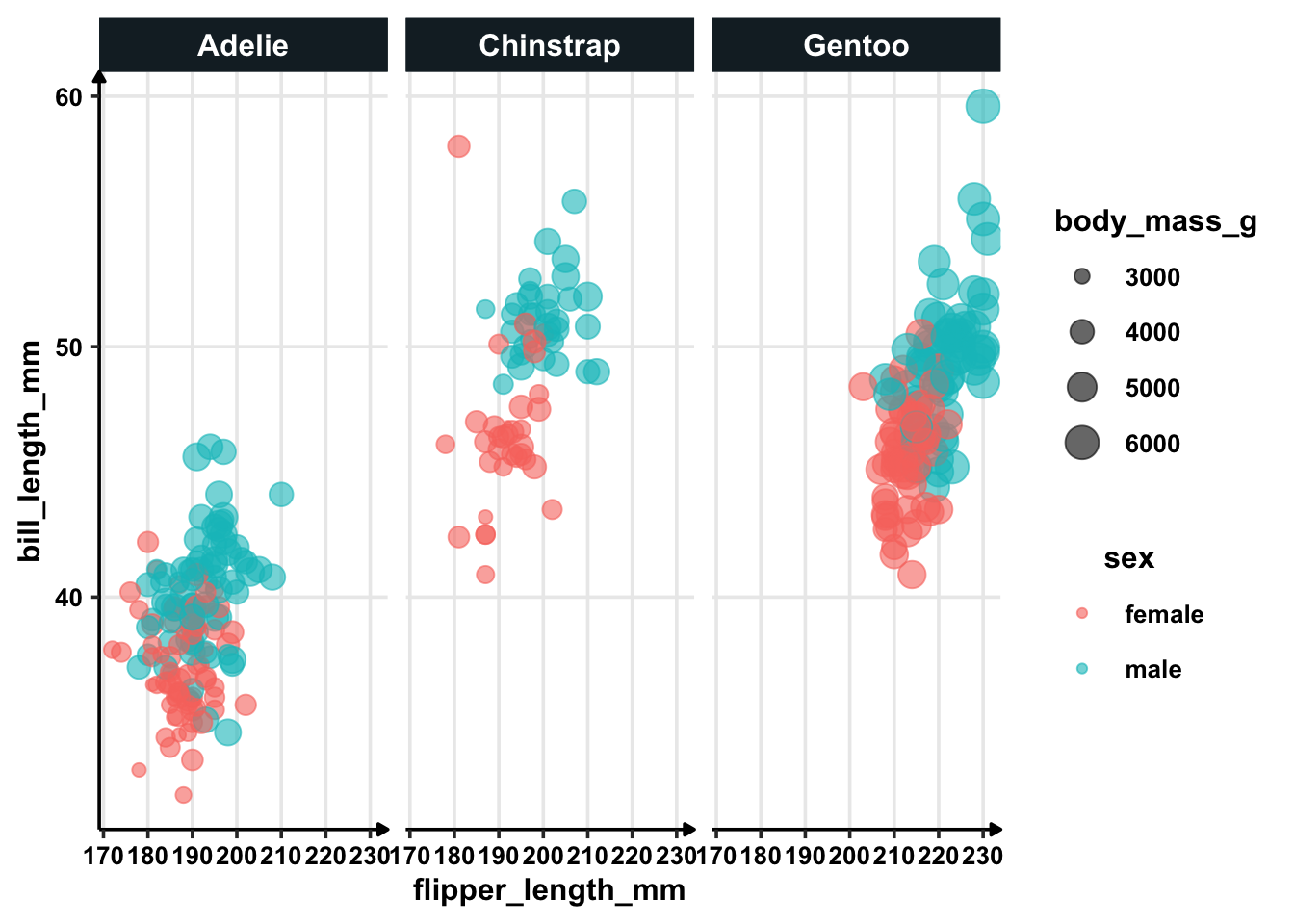
In general, there is significant difference between bill_length_mm for both the sexes. Also, bill length for Adelie is shorter than other two species — for moth the sexes.
There are also packages like DataExplorer that can aid in the process. For this simplistic case, I want to demonstrate how to create classification model, so I will ignore the process.
The dataset has missing values as I noted earlier. So, I will remove the observations with missing values. I also do not need year and island for my classification model — there is no logical reason why should they be affecting sex of a penguin.
penguins_df = penguins %>%
   filter(!is.na(sex)) %>%
   select(-year, -island)
Modelling
Let’s start by loading tidymodels and setting the seed for randomisation.
library(tidymodels)## ── Attaching packages ────────────────────────────────────── tidymodels 1.1.1 ──## ✔ broom 1.0.5 ✔ rsample 1.2.0
## ✔ dials 1.2.0 ✔ tune 1.1.2
## ✔ infer 1.0.4 ✔ workflows 1.1.3
## ✔ modeldata 1.2.0 ✔ workflowsets 1.0.1
## ✔ parsnip 1.1.1 ✔ yardstick 1.2.0
## ✔ recipes 1.0.8## ── Conflicts ───────────────────────────────────────── tidymodels_conflicts() ──
## ✖ scales::discard() masks purrr::discard()
## ✖ dplyr::filter() masks stats::filter()
## ✖ recipes::fixed() masks stringr::fixed()
## ✖ dplyr::lag() masks stats::lag()
## ✖ yardstick::spec() masks readr::spec()
## ✖ recipes::step() masks stats::step()
## • Learn how to get started at https://www.tidymodels.org/start/set.seed(1)The first step of modelling is to create the training and testing split. Validation set will never be exposed to us during the modelling process. Once our final model is made, we can test it against the validation set.
In Tidy Models, this split is created using initial_split function. I also have the option to stratify the split — which is necessary because we have multiple species and they are unbalanced. We only have 68 Chinstrap penguins but have 152 Adelie and 124 Gentoo. Let’s explore the help file for initial_split too.
?initial_split

# Specify the split
penguins_split = initial_split(penguins_df, strata = sex)
The proportion is set by default to 75% in training and 25% in testing. The functions training() and testing() will give me the resulting datasets.
penguins_train = training(penguins_split)
penguins_test = testing(penguins_split)

penguins_train
## # A tibble: 249 × 6
## species bill_length_mm bill_depth_mm flipper_length_mm body_mass_g sex
## <fct> <dbl> <dbl> <int> <int> <fct>
## 1 Adelie 39.5 17.4 186 3800 female
## 2 Adelie 40.3 18 195 3250 female
## 3 Adelie 36.7 19.3 193 3450 female
## 4 Adelie 36.6 17.8 185 3700 female
## 5 Adelie 38.7 19 195 3450 female
## 6 Adelie 35.9 19.2 189 3800 female
## 7 Adelie 37.9 18.6 172 3150 female
## 8 Adelie 39.5 16.7 178 3250 female
## 9 Adelie 39.5 17.8 188 3300 female
## 10 Adelie 42.2 18.5 180 3550 female
## # ℹ 239 more rowspenguins_test## # A tibble: 84 × 6
## species bill_length_mm bill_depth_mm flipper_length_mm body_mass_g sex
## <fct> <dbl> <dbl> <int> <int> <fct>
## 1 Adelie 38.9 17.8 181 3625 female
## 2 Adelie 39.2 19.6 195 4675 male
## 3 Adelie 41.1 17.6 182 3200 female
## 4 Adelie 34.4 18.4 184 3325 female
## 5 Adelie 46 21.5 194 4200 male
## 6 Adelie 37.8 18.3 174 3400 female
## 7 Adelie 37.7 18.7 180 3600 male
## 8 Adelie 35.3 18.9 187 3800 female
## 9 Adelie 40.6 18.6 183 3550 male
## 10 Adelie 40.5 17.9 187 3200 female
## # ℹ 74 more rowsThe datasets looks good; our split worked well.
Bootstrapping Samples
Note that our training sample has only 249 rows. This is not a huge dataset and we are not sure if the model we will make from this will be generalisable.
One simple way to solve this is using Bootstrapped samples. Each bootstrap sample is of original sample size but is also different from each other. They are collected sample of observations with replacement. Again, see the help file to understand the function.
?bootstraps

penguins_boot = bootstraps(penguins_train)
penguins_boot
## # Bootstrap sampling
## # A tibble: 25 × 2
## splits id
## <list> <chr>
## 1 <split [249/85]> Bootstrap01
## 2 <split [249/93]> Bootstrap02
## 3 <split [249/85]> Bootstrap03
## 4 <split [249/93]> Bootstrap04
## 5 <split [249/84]> Bootstrap05
## 6 <split [249/87]> Bootstrap06
## 7 <split [249/88]> Bootstrap07
## 8 <split [249/92]> Bootstrap08
## 9 <split [249/93]> Bootstrap09
## 10 <split [249/86]> Bootstrap10
## # ℹ 15 more rowsSo, we have 25 bootstrapped samples each with different resamples. Of course, if you have enough data or are confident enough about your data, you can skip this step.
Logistic Regression Pipeline
Logistic regression model is one of the simplest classification model. It is also the basic building block of neural networks; it dictates how a node behaves. Until 2010 when neural networks and support vector machines gained popularity, logistic regression was the model in force.
Even today, the model is widely used in variety of real world applications. The biggest benefit of logistic regression models is its ability to explain and linear implementation.
The first step will be to set up model pipeline. This only sets up how the model would work and neither training or test has happened yet.
# Simple Logistic Regression
glm_spec = logistic_reg() %>%
   set_engine("glm")

glm_spec
## Logistic Regression Model Specification (classification)
##
## Computational engine: glmThere are other alternatives too. We can use Lasso regression (yes, Lasso can be used for classification as well. It “estimate[s] the parameters of the binomial GLM by optimising the binomial likelihood whilst imposing the lasso penalty on the parameter estimates”.) Or we can just use a regularised classification model.
# regularised regression
glm_spec = logistic_reg() %>%
   set_engine("glmnet")

# LASSO regression
glm_spec = logistic_reg(mixture = 1) %>%
   set_engine("glmnet")
But for this simple tutorial, I will stick to simple logistic regression model.
# Simple Logistic Regression
glm_spec = logistic_reg() %>%
   set_engine("glm")
Random Forest Pipeline
Let’s set up a pipeline for random forest model as well. The good part about random forest model is that they do not require huge tuning efforts like neural networks.
Random forest models can be used for classification as well as regression. Furthermore, there are many implementations (packages) in R to choose from. randomForest is probably the most known one. ranger is a fast implementation of random forest models in R. I will use ranger for this model.
# Engine could be spark
rand_forest() %>%
   set_mode("classification") %>%
   set_engine("spark")
## Random Forest Model Specification (classification)
##
## Computational engine: spark# Or it could be randomForest
rand_forest() %>%
set_mode("classification") %>%
set_engine("randomForest")## Random Forest Model Specification (classification)
##
## Computational engine: randomForest# Or ranger
rf_spec = rand_forest() %>%
set_mode("classification") %>%
set_engine("ranger")
rf_spec## Random Forest Model Specification (classification)
##
## Computational engine: rangerWorkflow
The next step in modelling pipeline is setting up the model with formula, model and data — in that order. Because I have multiple models that I want to compare, I will only set up formula in my workflow.
penguin_wf = workflow() %>%
   add_formula(sex ~ .)
penguin_wf
## ══ Workflow ════════════════════════════════════════════════════════════════════
## Preprocessor: Formula
## Model: None
##
## ── Preprocessor ────────────────────────────────────────────────────────────────
## sex ~ .As it is seen, there is no model set yet.
Training Logistic Regression
Let’s add logistic regression model. I can fit it directly to the training sample.
penguin_wf %>%
   add_model(glm_spec) %>%
   fit(data = penguins_train)
## ══ Workflow [trained] ══════════════════════════════════════════════════════════
## Preprocessor: Formula
## Model: logistic_reg()
##
## ── Preprocessor ────────────────────────────────────────────────────────────────
## sex ~ .
##
## ── Model ───────────────────────────────────────────────────────────────────────
##
## Call: stats::glm(formula = ..y ~ ., family = stats::binomial, data = data)
##
## Coefficients:
## (Intercept) speciesChinstrap speciesGentoo bill_length_mm
## -95.852333 -6.932255 -8.535185 0.633832
## bill_depth_mm flipper_length_mm body_mass_g
## 2.014378 0.056401 0.006365
##
## Degrees of Freedom: 248 Total (i.e. Null); 242 Residual
## Null Deviance: 345.2
## Residual Deviance: 85.49 AIC: 99.49I get the coefficients and other detains for my model which is great.
However, as I said before I can’t be absolutely sure of my model right away because of small sample. So, I will use bootstrapped samples that I created earlier. verbose = T will show me all steps.
glm_rs = penguin_wf %>%
   add_model(glm_spec) %>%
   fit_resamples(resamples = penguins_boot,
                 control = control_resamples(save_pred = TRUE, verbose = F))
## → A | warning: glm.fit: fitted probabilities numerically 0 or 1 occurred## There were issues with some computations A: x1
## There were issues with some computations A: x1## glm_rs## # Resampling results
## # Bootstrap sampling
## # A tibble: 25 × 5
## splits id .metrics .notes .predictions
## <list> <chr> <list> <list> <list>
## 1 <split [249/85]> Bootstrap01 <tibble [2 × 4]> <tibble [0 × 3]> <tibble>
## 2 <split [249/93]> Bootstrap02 <tibble [2 × 4]> <tibble [0 × 3]> <tibble>
## 3 <split [249/85]> Bootstrap03 <tibble [2 × 4]> <tibble [0 × 3]> <tibble>
## 4 <split [249/93]> Bootstrap04 <tibble [2 × 4]> <tibble [0 × 3]> <tibble>
## 5 <split [249/84]> Bootstrap05 <tibble [2 × 4]> <tibble [0 × 3]> <tibble>
## 6 <split [249/87]> Bootstrap06 <tibble [2 × 4]> <tibble [0 × 3]> <tibble>
## 7 <split [249/88]> Bootstrap07 <tibble [2 × 4]> <tibble [0 × 3]> <tibble>
## 8 <split [249/92]> Bootstrap08 <tibble [2 × 4]> <tibble [0 × 3]> <tibble>
## 9 <split [249/93]> Bootstrap09 <tibble [2 × 4]> <tibble [0 × 3]> <tibble>
## 10 <split [249/86]> Bootstrap10 <tibble [2 × 4]> <tibble [0 × 3]> <tibble>
## # ℹ 15 more rows
##
## There were issues with some computations:
##
## - Warning(s) x1: glm.fit: fitted probabilities numerically 0 or 1 occurred
##
## Run `show_notes(.Last.tune.result)` for more information.One bootstrapped sample had sampling issues (they training labels were unbalanced). To solve this, I could have specified strata = sex in bootstraps(). In this case it is acceptable because 24 of them worked well.
Training Random Forest
The process is almost the same as that for logistic regression.
rf_rs = penguin_wf %>%
   add_model(rf_spec) %>%
   fit_resamples(resamples = penguins_boot,
                 control = control_resamples(save_pred = TRUE, verbose = F))

rf_rs
## # Resampling results
## # Bootstrap sampling
## # A tibble: 25 × 5
## splits id .metrics .notes .predictions
## <list> <chr> <list> <list> <list>
## 1 <split [249/85]> Bootstrap01 <tibble [2 × 4]> <tibble [0 × 3]> <tibble>
## 2 <split [249/93]> Bootstrap02 <tibble [2 × 4]> <tibble [0 × 3]> <tibble>
## 3 <split [249/85]> Bootstrap03 <tibble [2 × 4]> <tibble [0 × 3]> <tibble>
## 4 <split [249/93]> Bootstrap04 <tibble [2 × 4]> <tibble [0 × 3]> <tibble>
## 5 <split [249/84]> Bootstrap05 <tibble [2 × 4]> <tibble [0 × 3]> <tibble>
## 6 <split [249/87]> Bootstrap06 <tibble [2 × 4]> <tibble [0 × 3]> <tibble>
## 7 <split [249/88]> Bootstrap07 <tibble [2 × 4]> <tibble [0 × 3]> <tibble>
## 8 <split [249/92]> Bootstrap08 <tibble [2 × 4]> <tibble [0 × 3]> <tibble>
## 9 <split [249/93]> Bootstrap09 <tibble [2 × 4]> <tibble [0 × 3]> <tibble>
## 10 <split [249/86]> Bootstrap10 <tibble [2 × 4]> <tibble [0 × 3]> <tibble>
## # ℹ 15 more rowsNotice that I did not get the same warning in random forest model. Why? Because random forest is not probabilistic in nature. Tree based models do not necessitate presence of balanced samples. They will simply give biased results and it is up to the researcher to investigate the flaws. That’s why they are little tricky.
Evaluation
How well do they compare against each other? The metrics to compare can be obtained using collect_metrics().
Logistic Regression Metrics
collect_metrics(glm_rs)## # A tibble: 2 × 6
## .metric .estimator mean n std_err .config
## <chr> <chr> <dbl> <int> <dbl> <chr>
## 1 accuracy binary 0.905 25 0.00695 Preprocessor1_Model1
## 2 roc_auc binary 0.971 25 0.00291 Preprocessor1_Model1Random Forest Metrics
collect_metrics(rf_rs)## # A tibble: 2 × 6
## .metric .estimator mean n std_err .config
## <chr> <chr> <dbl> <int> <dbl> <chr>
## 1 accuracy binary 0.901 25 0.00629 Preprocessor1_Model1
## 2 roc_auc binary 0.970 25 0.00255 Preprocessor1_Model1Logistic regression performs slightly better in both metrics: accuracy and AUC. Even if they were nearly equal and I had to choose, I would choose linear model. It is faster to implement, scalable and most importantly explainable.
Predictions
The predictions can be found using collect_predictions() function.
glm_rs %>%
  collect_predictions()
## # A tibble: 2,250 × 7
## id .pred_female .pred_male .row .pred_class sex .config
## <chr> <dbl> <dbl> <int> <fct> <fct> <chr>
## 1 Bootstrap01 0.580 0.420 6 female female Preprocessor1_M…
## 2 Bootstrap01 0.987 0.0125 7 female female Preprocessor1_M…
## 3 Bootstrap01 0.978 0.0219 9 female female Preprocessor1_M…
## 4 Bootstrap01 0.0277 0.972 10 male female Preprocessor1_M…
## 5 Bootstrap01 0.842 0.158 11 female female Preprocessor1_M…
## 6 Bootstrap01 1.00 0.000350 12 female female Preprocessor1_M…
## 7 Bootstrap01 0.999 0.000525 13 female female Preprocessor1_M…
## 8 Bootstrap01 1.00 0.00000806 14 female female Preprocessor1_M…
## 9 Bootstrap01 0.918 0.0824 16 female female Preprocessor1_M…
## 10 Bootstrap01 0.966 0.0341 19 female female Preprocessor1_M…
## # ℹ 2,240 more rowsThe two important columns in this are .pred_female and .pred_male. This is the probability that they belong to a particular class. .pred_class gives the class that our model predicts a penguin to be in; sex is their true class.
Confusion Matrix
conf_mat_resampled() with no arguments gives confusion matrix in tidy format.
glm_rs %>%
  conf_mat_resampled()
## # A tibble: 4 × 3
## Prediction Truth Freq
## <fct> <fct> <dbl>
## 1 female female 39
## 2 female male 4.04
## 3 male female 4.44
## 4 male male 42.5Let’s see it in conventional format.
glm_rs %>%
  collect_predictions() %>%
  conf_mat(sex, .pred_class)
## Truth
## Prediction female male
## female 975 101
## male 111 1063The model looks pretty good.
ROC Curve
The ROC curve can be produced by roc_curve() function. autoplot() uses default settings.
glm_rs %>%
   collect_predictions() %>%
   group_by(id) %>% # -- to get 25 ROC curves, for each bootstrapped sample
   roc_curve(sex, .pred_female) %>%
   autoplot()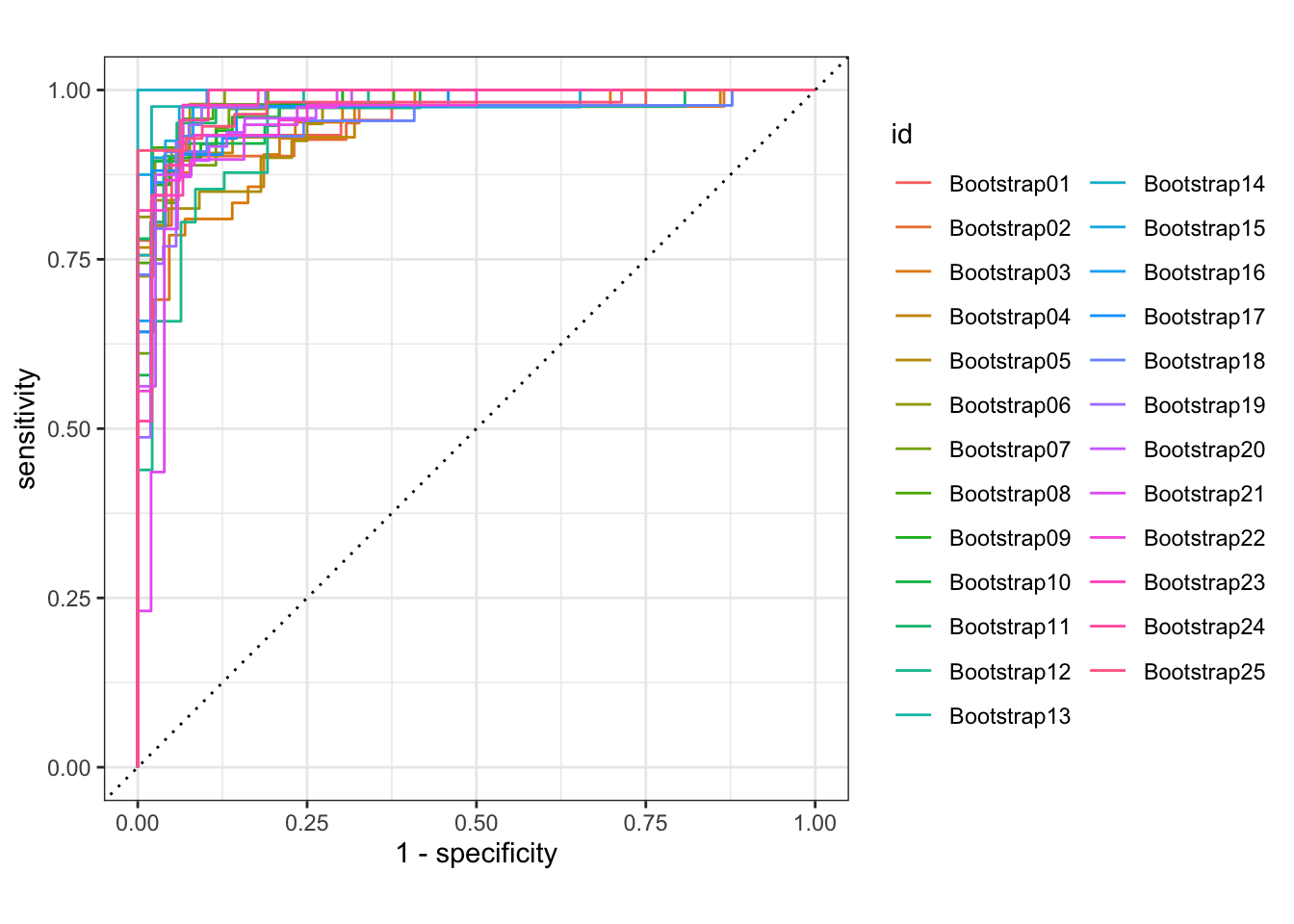
How does autoplot() work?
glm_rs %>%
   collect_predictions() %>%
   group_by(id) %>% # -- to get 25 ROC curves, for each bootstrapped sample
   roc_curve(sex, .pred_female)
## # A tibble: 2,296 × 4
## # Groups: id [25]
## id .threshold specificity sensitivity
## <chr> <dbl> <dbl> <dbl>
## 1 Bootstrap01 -Inf 0 1
## 2 Bootstrap01 6.67e-10 0 1
## 3 Bootstrap01 7.64e- 8 0.0250 1
## 4 Bootstrap01 8.21e- 8 0.0500 1
## 5 Bootstrap01 1.28e- 7 0.0750 1
## 6 Bootstrap01 1.58e- 7 0.1 1
## 7 Bootstrap01 3.33e- 6 0.125 1
## 8 Bootstrap01 1.42e- 5 0.15 1
## 9 Bootstrap01 1.49e- 5 0.175 1
## 10 Bootstrap01 2.19e- 5 0.2 1
## # ℹ 2,286 more rowsLet’s beautify our ROC curve.
glm_rs %>%
   collect_predictions() %>%
   group_by(id) %>% # -- to get 25 ROC curves, for each bootstrapped sample
   roc_curve(sex, .pred_female) %>%
   ggplot(aes(1 - specificity, sensitivity, col = id)) +
   geom_abline(lty = 2, colour = "grey80", size = 1.5) +
   geom_path(show.legend = FALSE, alpha = 0.6, size = 1.2) +
   coord_equal()
## Warning: Using `size` aesthetic for lines was deprecated in ggplot2 3.4.0.
## ℹ Please use `linewidth` instead.
## This warning is displayed once every 8 hours.
## Call `lifecycle::last_lifecycle_warnings()` to see where this warning was
## generated.
I’m using geom_path instead of geom_line because I want to see discrete jumps. geom_line would give me a continious plot as it connects the points in the order of the variable on the x-axis. Another option is geom_step which only highlights changes — when a variable steps to take another value.
# Using geom_line()
glm_rs %>%
   collect_predictions() %>%
   group_by(id) %>% # -- to get 25 ROC curves, for each bootstrapped sample
   roc_curve(sex, .pred_female) %>%
   ggplot(aes(1 - specificity, sensitivity, col = id)) +
   geom_abline(lty = 2, colour = "grey80", size = 1.5) +
   geom_line(show.legend = FALSE, alpha = 0.6, size = 1.2) +
   coord_equal()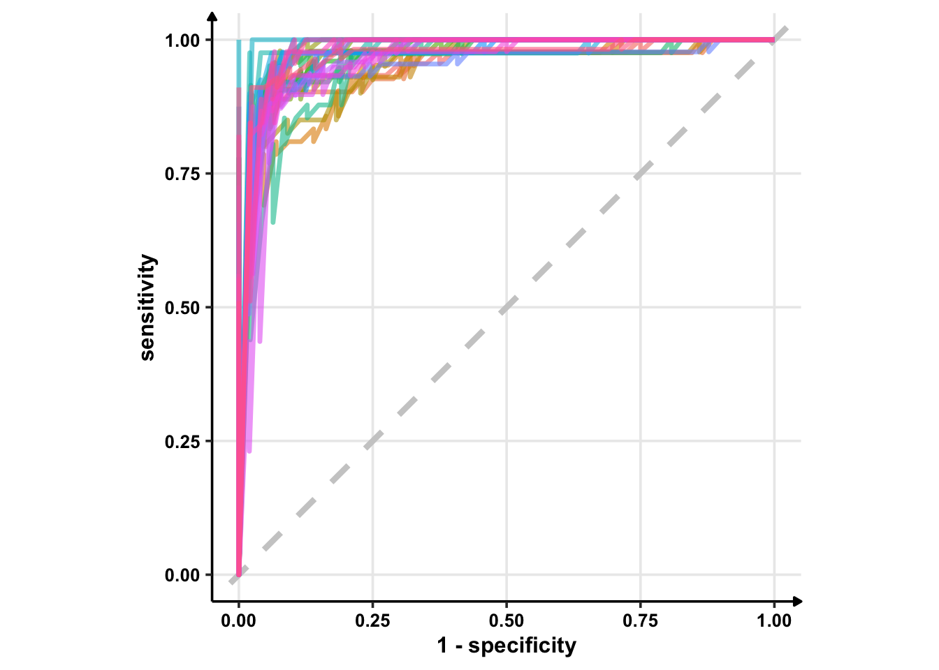
# Using geom_step()
glm_rs %>%
   collect_predictions() %>%
   group_by(id) %>% # -- to get 25 ROC curves, for each bootstrapped sample
   roc_curve(sex, .pred_female) %>%
   ggplot(aes(1 - specificity, sensitivity, col = id)) +
   geom_abline(lty = 2, colour = "grey80", size = 1.5) +
   geom_step(show.legend = FALSE, alpha = 0.6, size = 1.2) +
   coord_equal()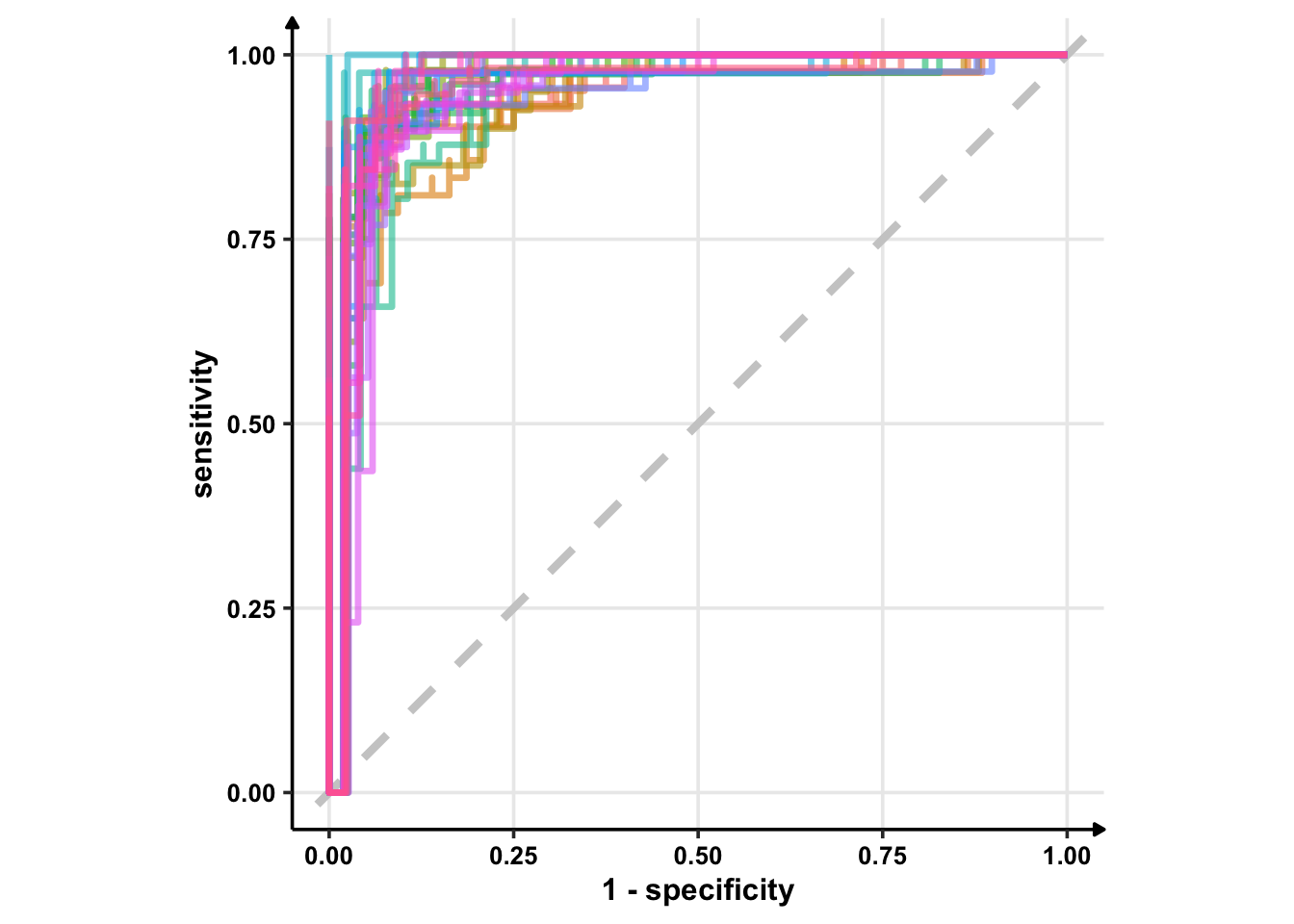
geom_abline() can take two arguments: intercept and slope. If you provide none of these, it plots \(y = x\). So, the best plot is from geom_path().
glm_rs %>%
   collect_predictions() %>%
   group_by(id) %>% # -- to get 25 ROC curves, for each bootstrapped sample
   roc_curve(sex, .pred_female) %>%
   ggplot(aes(1 - specificity, sensitivity, col = id)) +
   geom_abline(lty = 2, colour = "grey80", size = 1.5) +
   geom_path(show.legend = FALSE, alpha = 0.6, size = 1.2) +
   coord_equal()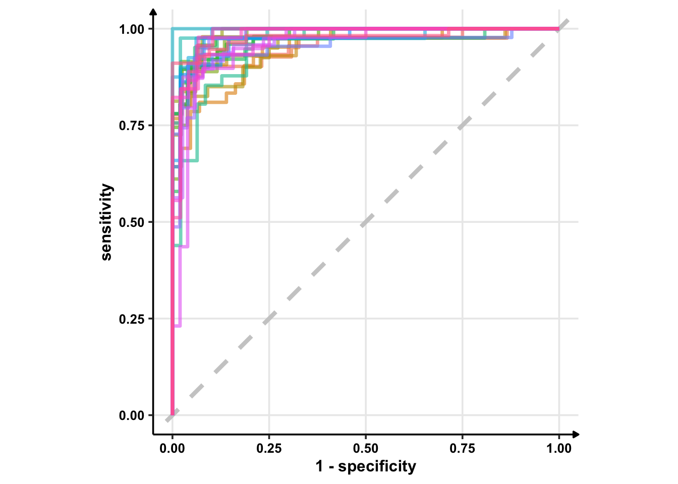
Okay, enough on ggplot2. From the above ROC curves, we can deduce the model is doing great for the training samples.
Testing Samples
The above metrics used only the test data. We need to check our model’s performance on test dataset too.
Let’s fit the model using last_fit(). last_fit() fits the final best model to the training set and evaluates the test set.
penguins_final = penguin_wf %>%
  add_model(glm_spec) %>%
  last_fit(penguins_split)

penguins_final
## # Resampling results
## # Manual resampling
## # A tibble: 1 × 6
## splits id .metrics .notes .predictions .workflow
## <list> <chr> <list> <list> <list> <list>
## 1 <split [249/84]> train/test split <tibble> <tibble> <tibble> <workflow>Let’s check how good our final model is.
penguins_final %>%
  collect_metrics()
## # A tibble: 2 × 4
## .metric .estimator .estimate .config
## <chr> <chr> <dbl> <chr>
## 1 accuracy binary 0.905 Preprocessor1_Model1
## 2 roc_auc binary 0.966 Preprocessor1_Model1penguins_final %>%
collect_predictions()## # A tibble: 84 × 7
## id .pred_female .pred_male .row .pred_class sex .config
## <chr> <dbl> <dbl> <int> <fct> <fct> <chr>
## 1 train/test split 0.887 0.113 6 female female Preprocess…
## 2 train/test split 0.0000979 1.00 7 male male Preprocess…
## 3 train/test split 0.976 0.0238 8 female female Preprocess…
## 4 train/test split 0.996 0.00431 14 female female Preprocess…
## 5 train/test split 0.000000623 1.00 15 male male Preprocess…
## 6 train/test split 0.973 0.0273 16 female female Preprocess…
## 7 train/test split 0.772 0.228 17 female male Preprocess…
## 8 train/test split 0.662 0.338 21 female female Preprocess…
## 9 train/test split 0.434 0.566 22 male male Preprocess…
## 10 train/test split 0.961 0.0388 23 female female Preprocess…
## # ℹ 74 more rowsOur model is 90.5% accurate and has AUC of 0.966. These are very high accuracies.
Confusion Matrix for Test Set
penguins_final %>%
collect_predictions() %>%
conf_mat(sex, .pred_class)## Truth
## Prediction female male
## female 39 5
## male 3 37This does pretty good to be honest.
Final Workflow
Let’s see the final model.
penguins_final$.workflow[[1]]## ══ Workflow [trained] ══════════════════════════════════════════════════════════
## Preprocessor: Formula
## Model: logistic_reg()
##
## ── Preprocessor ────────────────────────────────────────────────────────────────
## sex ~ .
##
## ── Model ───────────────────────────────────────────────────────────────────────
##
## Call: stats::glm(formula = ..y ~ ., family = stats::binomial, data = data)
##
## Coefficients:
## (Intercept) speciesChinstrap speciesGentoo bill_length_mm
## -95.852333 -6.932255 -8.535185 0.633832
## bill_depth_mm flipper_length_mm body_mass_g
## 2.014378 0.056401 0.006365
##
## Degrees of Freedom: 248 Total (i.e. Null); 242 Residual
## Null Deviance: 345.2
## Residual Deviance: 85.49 AIC: 99.49Can we tidy it up? (We need [[1]] to get the element out as .workflow is a list.
penguins_final$.workflow[[1]] %>%
  tidy()
## # A tibble: 7 × 5
## term estimate std.error statistic p.value
## <chr> <dbl> <dbl> <dbl> <dbl>
## 1 (Intercept) -95.9 18.1 -5.30 0.000000115
## 2 speciesChinstrap -6.93 1.91 -3.62 0.000295
## 3 speciesGentoo -8.54 3.25 -2.63 0.00866
## 4 bill_length_mm 0.634 0.159 4.00 0.0000639
## 5 bill_depth_mm 2.01 0.455 4.43 0.00000940
## 6 flipper_length_mm 0.0564 0.0653 0.863 0.388
## 7 body_mass_g 0.00637 0.00138 4.63 0.00000374The coefficients can be exponentiated to find the odds ratio.
penguins_final$.workflow[[1]] %>%
   tidy(exponentiate = TRUE) %>%
   arrange(estimate)
## # A tibble: 7 × 5
## term estimate std.error statistic p.value
## <chr> <dbl> <dbl> <dbl> <dbl>
## 1 (Intercept) 2.35e-42 18.1 -5.30 0.000000115
## 2 speciesGentoo 1.96e- 4 3.25 -2.63 0.00866
## 3 speciesChinstrap 9.76e- 4 1.91 -3.62 0.000295
## 4 body_mass_g 1.01e+ 0 0.00138 4.63 0.00000374
## 5 flipper_length_mm 1.06e+ 0 0.0653 0.863 0.388
## 6 bill_length_mm 1.88e+ 0 0.159 4.00 0.0000639
## 7 bill_depth_mm 7.50e+ 0 0.455 4.43 0.00000940The coefficient of 3.75 means that for every one mm increase in bill depth, the odds of being male increases by almost eight times. So, bill depth is very important.
Flipper value are not very important. Remember that previously we explored the relationship between sex and flipper length. If flipper length is not important (high p-value), let’s see how the graph would look like with bill depth which is apparently very important.
penguins %>%
   filter(!is.na(sex)) %>%
   ggplot(aes(bill_depth_mm, bill_length_mm, colour = sex, size = body_mass_g)) +
   geom_point(alpha = 0.6) +
   facet_wrap(~species)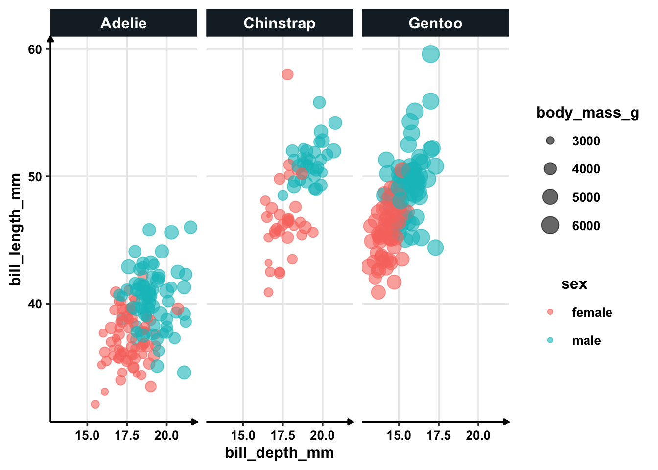
Conclusion
In this creating this short tutorial, I learnt how to classify data using tidymodels workflow with logistic regression and random forest. An important lesson was that logistic regression can outperform complicated trees like random forest too.
If you are interested in data science and R, check out my free weekly newsletter Next.
Next — Today I Learnt About R
A short and sweet curated collection of R-related works. Five stories. Four packages. Three jargons. Two tweets. One Meme.
You can read the past editions and subscribe to it here.